
77. Neural Machine Translation and Dialogue Systems#
77.1. Introduction#
Previously, we explained the recurrent neural network and introduced some of its applications in natural language processing. In this experiment, we will explain a variant of the recurrent neural network, namely the sequence-to-sequence model, which has been widely used in many tasks in natural language processing and achieved good results.
77.2. Key Points#
Sequence-to-Sequence Model
Neural Machine Translation System
Chatbot System
Natural language processing involves many fields, such as building dialogue systems, recommendation systems, and neural machine translation. These applications often require a lot of professional knowledge and tend to be research-oriented rather than beginner-applied. In the previous experiment, we focused on introducing feature extraction and text classification in natural language processing. In this experiment, we will introduce the sequence-to-sequence model and conduct a preliminary exploration of its applications in machine translation and dialogue systems.
77.3. Sequence-to-Sequence Model#
The Sequence to Sequence model, abbreviated as seq2seq, is a model composed of an encoder and a decoder. This model was first proposed in 2014 by Kyunghyun Cho, a member of the team led by Yoshua Bengio, and it mainly addresses the problem of dealing with variable-length input sequences and variable-length output sequences.
Professor Yoshua Bengio is the third person from the left in the following picture. Do you know the other three big names? 😏
Let’s first review the recurrent neural networks learned previously. When explaining recurrent neural networks, we mentioned that there are mainly the following types when dealing with sequence problems, namely:
-
1 → N: Generation model, that is, input a vector and output a sequence of length N.
-
N → 1: Discriminative model, that is, input a sequence of length N and output a vector.
-
N → N: Standard sequence model, that is, input a sequence of length N and output a sequence of length N.
-
N → M: Variable-length sequence model, that is, input a sequence of length N and output a sequence of length M.
For the standard recurrent neural network, it can only solve the first three problem types listed above, namely 1 to N, N to 1, and N to N. In other words, if the input sequence and the output sequence are not equal, the standard recurrent neural network cannot be used for modeling. To solve this problem, Kyunghyun Cho et al. proposed the encoder model and the decoder model, as shown in the following figure:
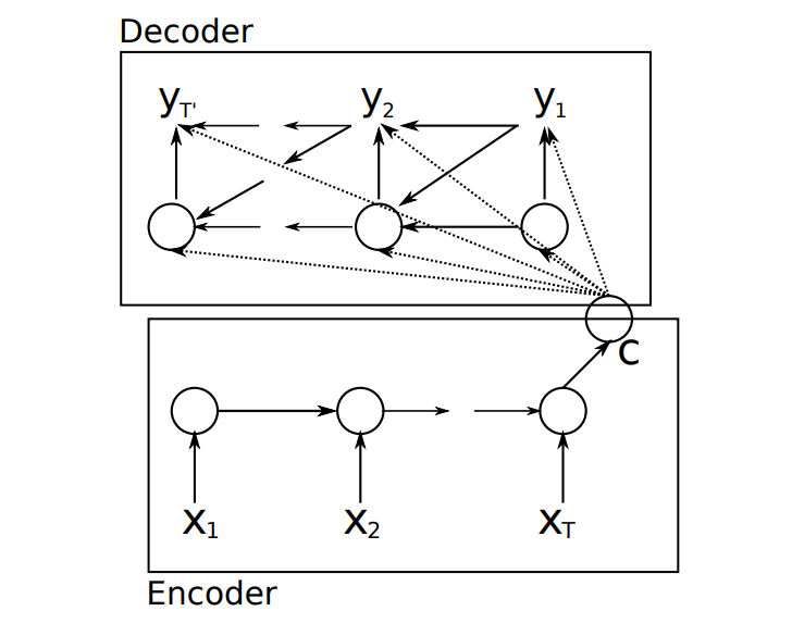
In the figure, \(X_{i}\) represents the input sequence, \(y_{i}\) represents the output sequence, and \(C\) represents the output state after encoding the input sequence. From the above figure, we can see that this model is mainly composed of an encoder and a decoder. When we input the sequence \(X_{i}\), it is encoded by a recurrent neural network to obtain a state vector \(C\). The decoder is also a recurrent neural network, which decodes through the state \(C\) obtained by the encoder to obtain a set of output sequences.
For ease of understanding, the experiment gives a simple example to illustrate. Suppose we now want to build a machine translation system for Chinese to English, and the sentence to be translated is as follows:
Chinese: 我有一个苹果 English: I have a apple
For the machine translation task, we can build a model as shown in the following figure.

In the figure shown above, the Chinese text to be translated consists of 6 characters, and the length of the input sequence is 6. The translation result is 4 words, so the length of the output sequence is 4. When we input the sentence “我有一个苹果” into the seq2seq model, the model will extract the features of the input sentence through a recurrent neural network and then encode them into a state vector. Then, this vector is used as the initial state value of the decoder. The decoder is also a recurrent neural network, and the output at each moment of the recurrent neural network is the translation result we want.
77.4. Neural Machine Translation System#
Previously, the principle of the seq2seq model was mainly explained. Now, we will implement a machine translation system to deepen our understanding. Before introducing the machine translation system, let’s briefly introduce machine translation.

Machine translation, as the name implies, is to translate one language into another through a computer. Currently, it mainly includes: rule-based methods, statistic-based methods, and neural network-based methods.
Before 2013, rule-based and statistical model-based machine translation were the mainstream methods. If you are interested, you can read [Statistical Natural Language Processing] (https://book.douban.com/subject/3076996/) written by Professor Zong Chengqing. After 2013, neural network-based machine translation (NMT, Neural Machine Translation) gradually emerged. Compared with previous statistical models, neural network machine translation has the advantages of fluent translations, accurate and easy-to-understand translations, and fast translation speeds. Therefore, the neural network-based method has gradually gained the favor of many scholars.
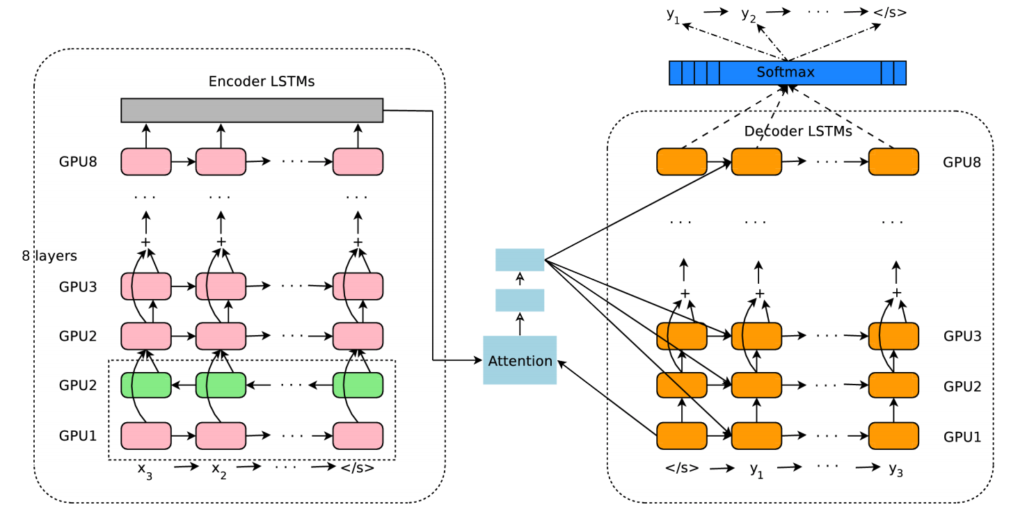
At the end of 2016, Google developed and launched Google’s Neural Machine Translation, and neural network machine translation officially stepped onto the stage. The following figure shows the neural network model of Google Translate. It is mainly composed of an encoder and a decoder, and both the encoder and the decoder use 8-layer recurrent neural networks.
However, such commercial neural machine translation systems are all too complex. Next, we will experimentally implement a small machine translation system.
77.4.1. Data Construction and Preprocessing#
The excellent performance of neural machine translation systems depends on large-scale corpus data. In this experiment, we only use a few simple Chinese-English corpora for demonstration. The key point for everyone is to understand the idea of neural machine translation and the principle of the seq2seq method.
input_texts = [
    "我有一个苹果",
    "你好吗",
    "见到你很高兴",
    "我简直不敢相信",
    "我知道那种感觉",
    "我真的非常后悔",
    "我也这样以为",
    "这样可以吗",
    "这事可能发生在任何人身上",
    "我想要一个手机",
]
output_texts = [
    "I have a apple",
    "How are you",
    "Nice to meet you",
    "I can not believe it",
    "I know the feeling",
    "I really regret it",
    "I thought so, too",
    "Is that OK",
    "It can happen to anyone",
    "I want a iphone",
]
Generally, for Chinese sentences, they are usually tokenized first before subsequent processing. However, since only a few sentences are used in the experiment, for convenience, each character is directly treated as a word. Now, we perform deduplication and statistics on the characters that appear in the input sentences.
def count_char(input_texts):
    input_characters = set()  # 用来存放输入集出现的中文字
    for input_text in input_texts:  # 遍历输入集的每一个句子
        for char in input_text:  # 遍历每个句子的每个字
            if char not in input_characters:
                input_characters.add(char)
    return input_characters


input_characters = count_char(input_texts)
input_characters
{'一',
 '上',
 '不',
 '个',
 '为',
 '也',
 '事',
 '人',
 '以',
 '任',
 '何',
 '你',
 '信',
 '兴',
 '到',
 '发',
 '可',
 '后',
 '吗',
 '在',
 '好',
 '常',
 '很',
 '悔',
 '想',
 '感',
 '我',
 '手',
 '敢',
 '有',
 '机',
 '果',
 '样',
 '生',
 '的',
 '直',
 '相',
 '真',
 '知',
 '种',
 '简',
 '能',
 '苹',
 '要',
 '见',
 '觉',
 '身',
 '这',
 '道',
 '那',
 '非',
 '高'}
Next, use the same method to perform statistics on the
output English sentences. It should be noted that the
sentence start marker
>
and the sentence end marker
<
are added to each output sentence.
def count_word(output_texts):
    target_characters = set()  # 用来存放输出集出现的单词
    target_texts = []  # 存放加了句子开头和结尾标记的句子
    for target_text in output_texts:  # 遍历输出集的每个句子
        target_text = "> " + target_text + " <"
        target_texts.append(target_text)
        word_list = target_text.split(" ")  # 对每个英文句子按空格划分,得到每个单词
        for word in word_list:  # 遍历每个单词
            if word not in target_characters:
                target_characters.add(word)
    return target_texts, target_characters


target_texts, target_characters = count_word(output_texts)
target_texts, target_characters
(['> I have a apple <',
  '> How are you <',
  '> Nice to meet you <',
  '> I can not believe it <',
  '> I know the feeling <',
  '> I really regret it <',
  '> I thought so, too <',
  '> Is that OK <',
  '> It can happen to anyone <',
  '> I want a iphone <'],
 {'<',
  '>',
  'How',
  'I',
  'Is',
  'It',
  'Nice',
  'OK',
  'a',
  'anyone',
  'apple',
  'are',
  'believe',
  'can',
  'feeling',
  'happen',
  'have',
  'iphone',
  'it',
  'know',
  'meet',
  'not',
  'really',
  'regret',
  'so,',
  'that',
  'the',
  'thought',
  'to',
  'too',
  'want',
  'you'})
Then, the experiment serializes the characters by creating a dictionary. After all, computers cannot directly understand human language.
input_characters = sorted(list(input_characters))  # 这里排序是为了每一次
target_characters = sorted(list(target_characters))  # 构建的字典都一样
# 构建字符到数字的字典,每个字符对应一个数字
input_token_index = dict([(char, i) for i, char in enumerate(input_characters)])
target_token_index = dict([(char, i) for i, char in enumerate(target_characters)])

input_token_index
{'一': 0,
 '上': 1,
 '不': 2,
 '个': 3,
 '为': 4,
 '也': 5,
 '事': 6,
 '人': 7,
 '以': 8,
 '任': 9,
 '何': 10,
 '你': 11,
 '信': 12,
 '兴': 13,
 '到': 14,
 '发': 15,
 '可': 16,
 '后': 17,
 '吗': 18,
 '在': 19,
 '好': 20,
 '常': 21,
 '很': 22,
 '悔': 23,
 '想': 24,
 '感': 25,
 '我': 26,
 '手': 27,
 '敢': 28,
 '有': 29,
 '机': 30,
 '果': 31,
 '样': 32,
 '生': 33,
 '的': 34,
 '直': 35,
 '相': 36,
 '真': 37,
 '知': 38,
 '种': 39,
 '简': 40,
 '能': 41,
 '苹': 42,
 '要': 43,
 '见': 44,
 '觉': 45,
 '身': 46,
 '这': 47,
 '道': 48,
 '那': 49,
 '非': 50,
 '高': 51}
Similarly, the experiment needs to define a dictionary that converts numerical values into characters for future use.
# 构建反向字典,每个数字对应一个字符
reverse_input_char_index = dict((i, char) for char, i in input_token_index.items())

reverse_target_char_index = dict((i, char) for char, i in target_token_index.items())

reverse_input_char_index
{0: '一',
 1: '上',
 2: '不',
 3: '个',
 4: '为',
 5: '也',
 6: '事',
 7: '人',
 8: '以',
 9: '任',
 10: '何',
 11: '你',
 12: '信',
 13: '兴',
 14: '到',
 15: '发',
 16: '可',
 17: '后',
 18: '吗',
 19: '在',
 20: '好',
 21: '常',
 22: '很',
 23: '悔',
 24: '想',
 25: '感',
 26: '我',
 27: '手',
 28: '敢',
 29: '有',
 30: '机',
 31: '果',
 32: '样',
 33: '生',
 34: '的',
 35: '直',
 36: '相',
 37: '真',
 38: '知',
 39: '种',
 40: '简',
 41: '能',
 42: '苹',
 43: '要',
 44: '见',
 45: '觉',
 46: '身',
 47: '这',
 48: '道',
 49: '那',
 50: '非',
 51: '高'}
Next, we calculate the number of input characters and output words respectively, for the subsequent one-hot encoding of input sentences and output sentences. At the same time, we calculate the length of the longest input sentence and the length of the longest output sentence respectively.
num_encoder_tokens = len(input_characters)  # 输入集不重复的字数
num_decoder_tokens = len(target_characters)  # 输出集不重复的单词数
max_encoder_seq_length = max([len(txt) for txt in input_texts])  # 输入集最长句子的长度
max_decoder_seq_length = max([len(txt) for txt in target_texts])  # 输出集最长句子的长度
Then, both the input sentences and the output sentences need to be converted into vector forms. It should be noted here that we convert the output sentences into two pieces of data, one is the original output sentence sequence, and the other is the sequence of the output sentences delayed by one time step. The two sequences serve as the input and output of the decoder respectively.
import numpy as np

# 创三个全为 0 的三维矩阵,第一维为样本数,第二维为句最大句子长度,第三维为每个字符的独热编码。
encoder_input_data = np.zeros(
    (len(input_texts), max_encoder_seq_length, num_encoder_tokens), dtype="float32"
)
decoder_input_data = np.zeros(
    (len(input_texts), max_decoder_seq_length, num_decoder_tokens), dtype="float32"
)
decoder_target_data = np.zeros(
    (len(input_texts), max_decoder_seq_length, num_decoder_tokens), dtype="float32"
)

for i, (input_text, target_text) in enumerate(
    zip(input_texts, target_texts)
):  # 遍历输入集和输出集
    for t, char in enumerate(input_text):  # 遍历输入集每个句子
        encoder_input_data[i, t, input_token_index[char]] = 1.0  # 字符对应的位置等于 1
    for t, char in enumerate(target_text.split(" ")):  # 遍历输出集的每个单词
        # 解码器的输入序列
        decoder_input_data[i, t, target_token_index[char]] = 1.0
        if t > 0:
            # 解码器的输出序列
            decoder_target_data[i, t - 1, target_token_index[char]] = 1.0
In the above code,
decoder_input_data
represents the input sequence of the decoder, for example:
【> I have a apple】. And
decoder_target_data
represents the output sequence of the decoder, for
example: 【I have a apple <】.
Take a look at the results of one-hot encoding:
encoder_input_data[0]
array([[0., 0., 0., 0., 0., 0., 0., 0., 0., 0., 0., 0., 0., 0., 0., 0.,
        0., 0., 0., 0., 0., 0., 0., 0., 0., 0., 1., 0., 0., 0., 0., 0.,
        0., 0., 0., 0., 0., 0., 0., 0., 0., 0., 0., 0., 0., 0., 0., 0.,
        0., 0., 0., 0.],
       [0., 0., 0., 0., 0., 0., 0., 0., 0., 0., 0., 0., 0., 0., 0., 0.,
        0., 0., 0., 0., 0., 0., 0., 0., 0., 0., 0., 0., 0., 1., 0., 0.,
        0., 0., 0., 0., 0., 0., 0., 0., 0., 0., 0., 0., 0., 0., 0., 0.,
        0., 0., 0., 0.],
       [1., 0., 0., 0., 0., 0., 0., 0., 0., 0., 0., 0., 0., 0., 0., 0.,
        0., 0., 0., 0., 0., 0., 0., 0., 0., 0., 0., 0., 0., 0., 0., 0.,
        0., 0., 0., 0., 0., 0., 0., 0., 0., 0., 0., 0., 0., 0., 0., 0.,
        0., 0., 0., 0.],
       [0., 0., 0., 1., 0., 0., 0., 0., 0., 0., 0., 0., 0., 0., 0., 0.,
        0., 0., 0., 0., 0., 0., 0., 0., 0., 0., 0., 0., 0., 0., 0., 0.,
        0., 0., 0., 0., 0., 0., 0., 0., 0., 0., 0., 0., 0., 0., 0., 0.,
        0., 0., 0., 0.],
       [0., 0., 0., 0., 0., 0., 0., 0., 0., 0., 0., 0., 0., 0., 0., 0.,
        0., 0., 0., 0., 0., 0., 0., 0., 0., 0., 0., 0., 0., 0., 0., 0.,
        0., 0., 0., 0., 0., 0., 0., 0., 0., 0., 1., 0., 0., 0., 0., 0.,
        0., 0., 0., 0.],
       [0., 0., 0., 0., 0., 0., 0., 0., 0., 0., 0., 0., 0., 0., 0., 0.,
        0., 0., 0., 0., 0., 0., 0., 0., 0., 0., 0., 0., 0., 0., 0., 1.,
        0., 0., 0., 0., 0., 0., 0., 0., 0., 0., 0., 0., 0., 0., 0., 0.,
        0., 0., 0., 0.],
       [0., 0., 0., 0., 0., 0., 0., 0., 0., 0., 0., 0., 0., 0., 0., 0.,
        0., 0., 0., 0., 0., 0., 0., 0., 0., 0., 0., 0., 0., 0., 0., 0.,
        0., 0., 0., 0., 0., 0., 0., 0., 0., 0., 0., 0., 0., 0., 0., 0.,
        0., 0., 0., 0.],
       [0., 0., 0., 0., 0., 0., 0., 0., 0., 0., 0., 0., 0., 0., 0., 0.,
        0., 0., 0., 0., 0., 0., 0., 0., 0., 0., 0., 0., 0., 0., 0., 0.,
        0., 0., 0., 0., 0., 0., 0., 0., 0., 0., 0., 0., 0., 0., 0., 0.,
        0., 0., 0., 0.],
       [0., 0., 0., 0., 0., 0., 0., 0., 0., 0., 0., 0., 0., 0., 0., 0.,
        0., 0., 0., 0., 0., 0., 0., 0., 0., 0., 0., 0., 0., 0., 0., 0.,
        0., 0., 0., 0., 0., 0., 0., 0., 0., 0., 0., 0., 0., 0., 0., 0.,
        0., 0., 0., 0.],
       [0., 0., 0., 0., 0., 0., 0., 0., 0., 0., 0., 0., 0., 0., 0., 0.,
        0., 0., 0., 0., 0., 0., 0., 0., 0., 0., 0., 0., 0., 0., 0., 0.,
        0., 0., 0., 0., 0., 0., 0., 0., 0., 0., 0., 0., 0., 0., 0., 0.,
        0., 0., 0., 0.],
       [0., 0., 0., 0., 0., 0., 0., 0., 0., 0., 0., 0., 0., 0., 0., 0.,
        0., 0., 0., 0., 0., 0., 0., 0., 0., 0., 0., 0., 0., 0., 0., 0.,
        0., 0., 0., 0., 0., 0., 0., 0., 0., 0., 0., 0., 0., 0., 0., 0.,
        0., 0., 0., 0.],
       [0., 0., 0., 0., 0., 0., 0., 0., 0., 0., 0., 0., 0., 0., 0., 0.,
        0., 0., 0., 0., 0., 0., 0., 0., 0., 0., 0., 0., 0., 0., 0., 0.,
        0., 0., 0., 0., 0., 0., 0., 0., 0., 0., 0., 0., 0., 0., 0., 0.,
        0., 0., 0., 0.]], dtype=float32)
After completing the above data preprocessing work, now let’s build a seq2seq model. In this experiment, TensorFlow Keras is used to build the model.
When training the seq2seq model, the model encodes the input Chinese sentence to obtain a state value, which also preserves the information of the Chinese sentence. In the decoder network, the state value obtained by the encoder is used as the initial state value input of the decoder.
In addition, the corpus data has each Chinese sentence corresponding to an English sentence. The Chinese sentence is used as the input of the encoder, and the English sentence is used as the output of the decoder. However, in the decoder, an input is also required. Here, the current word is used as the input, and the next word is selected as the output. As shown in the following figure:

In the above figure, the
>
symbol in the decoder represents the start of the
sentence, and the
<
symbol represents the end of the sentence. That is to say,
for each English sentence in the dataset, the
start-of-sentence marker symbol
>
and the end symbol
<
need to be added. During training, our input data mainly
consists of two parts, namely the Chinese sentence
【我有一个苹果】 (I have an apple), the English sentence
【> I have a apple】, and the output sentence is only
one 【I have a apple <】.
According to the seq2seq model shown in the above figure, build the encoder model and the decoder model respectively. First, build the encoder model:
import tensorflow as tf

latent_dim = 256  # 循环神经网络的神经单元数

# 编码器模型
encoder_inputs = tf.keras.Input(shape=(None, num_encoder_tokens))  # 编码器的输入
encoder = tf.keras.layers.LSTM(latent_dim, return_state=True)
encoder_outputs, state_h, state_c = encoder(encoder_inputs)  # 编码器的输出

encoder_states = [state_h, state_c]  # 状态值
encoder_states
[<KerasTensor: shape=(None, 256) dtype=float32 (created by layer 'lstm')>,
 <KerasTensor: shape=(None, 256) dtype=float32 (created by layer 'lstm')>]
Here we use LSTM as the encoder and decoder, so the output of the encoder mainly contains two values, namely H and C. Now use these two values as the input of the initial state values of the decoder.
# 解码器模型
decoder_inputs = tf.keras.Input(shape=(None, num_decoder_tokens))  # 解码器输入
decoder_lstm = tf.keras.layers.LSTM(
    latent_dim, return_sequences=True, return_state=True
)

# 初始化解码模型的状态值为 encoder_states
decoder_outputs, _, _ = decoder_lstm(decoder_inputs, initial_state=encoder_states)

# 连接一层全连接层,并使用 Softmax 求出每个时刻的输出
decoder_dense = tf.keras.layers.Dense(num_decoder_tokens, activation="softmax")
decoder_outputs = decoder_dense(decoder_outputs)  # 解码器输出
decoder_outputs
<KerasTensor: shape=(None, None, 32) dtype=float32 (created by layer 'dense')>
After building the decoder, now combine the encoder and the decoder to form a complete seq2seq model.
# 定义训练模型
model = tf.keras.Model([encoder_inputs, decoder_inputs], decoder_outputs)
model.summary()
Model: "model"
__________________________________________________________________________________________________
 Layer (type)                Output Shape                 Param #   Connected to
==================================================================================================
 input_1 (InputLayer)        [(None, None, 52)]           0         []

 input_2 (InputLayer)        [(None, None, 32)]           0         []

 lstm (LSTM)                 [(None, 256),                316416    ['input_1[0][0]']
                              (None, 256),
                              (None, 256)]

 lstm_1 (LSTM)               [(None, None, 256),          295936    ['input_2[0][0]',
                              (None, 256),                           'lstm[0][1]',
                              (None, 256)]                           'lstm[0][2]']

 dense (Dense)               (None, None, 32)             8224      ['lstm_1[0][0]']

==================================================================================================
Total params: 620576 (2.37 MB)
Trainable params: 620576 (2.37 MB)
Non-trainable params: 0 (0.00 Byte)
__________________________________________________________________________________________________
Next, select the loss function and optimizer, compile the model, and complete the training.
# 定义优化算法和损失函数
model.compile(optimizer="adam", loss="categorical_crossentropy")

# 训练模型
model.fit(
    [encoder_input_data, decoder_input_data],
    decoder_target_data,
    batch_size=10,
    epochs=200,
)
Epoch 1/200
1/1 [==============================] - 1s 812ms/step - loss: 0.6418
Epoch 2/200
1/1 [==============================] - 0s 21ms/step - loss: 0.6394
Epoch 3/200
1/1 [==============================] - 0s 22ms/step - loss: 0.6370
Epoch 4/200
1/1 [==============================] - 0s 24ms/step - loss: 0.6345
Epoch 5/200
1/1 [==============================] - 0s 22ms/step - loss: 0.6320
Epoch 6/200
1/1 [==============================] - 0s 23ms/step - loss: 0.6293
Epoch 7/200
1/1 [==============================] - 0s 25ms/step - loss: 0.6265
Epoch 8/200
1/1 [==============================] - 0s 24ms/step - loss: 0.6236
Epoch 9/200
1/1 [==============================] - 0s 24ms/step - loss: 0.6202
Epoch 10/200
1/1 [==============================] - 0s 25ms/step - loss: 0.6157
Epoch 11/200
1/1 [==============================] - 0s 24ms/step - loss: 0.6090
Epoch 12/200
1/1 [==============================] - 0s 24ms/step - loss: 0.5997
Epoch 13/200
1/1 [==============================] - 0s 22ms/step - loss: 0.5908
Epoch 14/200
1/1 [==============================] - 0s 23ms/step - loss: 0.5896
Epoch 15/200
1/1 [==============================] - 0s 23ms/step - loss: 0.5937
Epoch 16/200
1/1 [==============================] - 0s 26ms/step - loss: 0.5934
Epoch 17/200
1/1 [==============================] - 0s 23ms/step - loss: 0.5878
Epoch 18/200
1/1 [==============================] - 0s 23ms/step - loss: 0.5832
Epoch 19/200
1/1 [==============================] - 0s 23ms/step - loss: 0.5827
Epoch 20/200
1/1 [==============================] - 0s 22ms/step - loss: 0.5810
Epoch 21/200
1/1 [==============================] - 0s 23ms/step - loss: 0.5729
Epoch 22/200
1/1 [==============================] - 0s 23ms/step - loss: 0.5602
Epoch 23/200
1/1 [==============================] - 0s 22ms/step - loss: 0.5480
Epoch 24/200
1/1 [==============================] - 0s 23ms/step - loss: 0.5394
Epoch 25/200
1/1 [==============================] - 0s 23ms/step - loss: 0.5340
Epoch 26/200
1/1 [==============================] - 0s 22ms/step - loss: 0.5307
Epoch 27/200
1/1 [==============================] - 0s 22ms/step - loss: 0.5283
Epoch 28/200
1/1 [==============================] - 0s 22ms/step - loss: 0.5263
Epoch 29/200
1/1 [==============================] - 0s 23ms/step - loss: 0.5239
Epoch 30/200
1/1 [==============================] - 0s 22ms/step - loss: 0.5211
Epoch 31/200
1/1 [==============================] - 0s 23ms/step - loss: 0.5185
Epoch 32/200
1/1 [==============================] - 0s 21ms/step - loss: 0.5167
Epoch 33/200
1/1 [==============================] - 0s 22ms/step - loss: 0.5153
Epoch 34/200
1/1 [==============================] - 0s 22ms/step - loss: 0.5140
Epoch 35/200
1/1 [==============================] - 0s 23ms/step - loss: 0.5126
Epoch 36/200
1/1 [==============================] - 0s 22ms/step - loss: 0.5113
Epoch 37/200
1/1 [==============================] - 0s 24ms/step - loss: 0.5102
Epoch 38/200
1/1 [==============================] - 0s 23ms/step - loss: 0.5090
Epoch 39/200
1/1 [==============================] - 0s 22ms/step - loss: 0.5077
Epoch 40/200
1/1 [==============================] - 0s 23ms/step - loss: 0.5064
Epoch 41/200
1/1 [==============================] - 0s 24ms/step - loss: 0.5051
Epoch 42/200
1/1 [==============================] - 0s 25ms/step - loss: 0.5038
Epoch 43/200
1/1 [==============================] - 0s 24ms/step - loss: 0.5025
Epoch 44/200
1/1 [==============================] - 0s 23ms/step - loss: 0.5013
Epoch 45/200
1/1 [==============================] - 0s 23ms/step - loss: 0.5003
Epoch 46/200
1/1 [==============================] - 0s 23ms/step - loss: 0.4995
Epoch 47/200
1/1 [==============================] - 0s 23ms/step - loss: 0.4987
Epoch 48/200
1/1 [==============================] - 0s 23ms/step - loss: 0.4980
Epoch 49/200
1/1 [==============================] - 0s 24ms/step - loss: 0.4971
Epoch 50/200
1/1 [==============================] - 0s 23ms/step - loss: 0.4958
Epoch 51/200
1/1 [==============================] - 0s 22ms/step - loss: 0.4943
Epoch 52/200
1/1 [==============================] - 0s 23ms/step - loss: 0.4928
Epoch 53/200
1/1 [==============================] - 0s 22ms/step - loss: 0.4915
Epoch 54/200
1/1 [==============================] - 0s 22ms/step - loss: 0.4902
Epoch 55/200
1/1 [==============================] - 0s 24ms/step - loss: 0.4889
Epoch 56/200
1/1 [==============================] - 0s 24ms/step - loss: 0.4877
Epoch 57/200
1/1 [==============================] - 0s 28ms/step - loss: 0.4863
Epoch 58/200
1/1 [==============================] - 0s 24ms/step - loss: 0.4847
Epoch 59/200
1/1 [==============================] - 0s 23ms/step - loss: 0.4828
Epoch 60/200
1/1 [==============================] - 0s 23ms/step - loss: 0.4810
Epoch 61/200
1/1 [==============================] - 0s 23ms/step - loss: 0.4795
Epoch 62/200
1/1 [==============================] - 0s 24ms/step - loss: 0.4781
Epoch 63/200
1/1 [==============================] - 0s 23ms/step - loss: 0.4766
Epoch 64/200
1/1 [==============================] - 0s 20ms/step - loss: 0.4748
Epoch 65/200
1/1 [==============================] - 0s 23ms/step - loss: 0.4726
Epoch 66/200
1/1 [==============================] - 0s 23ms/step - loss: 0.4706
Epoch 67/200
1/1 [==============================] - 0s 23ms/step - loss: 0.4689
Epoch 68/200
1/1 [==============================] - 0s 23ms/step - loss: 0.4673
Epoch 69/200
1/1 [==============================] - 0s 24ms/step - loss: 0.4655
Epoch 70/200
1/1 [==============================] - 0s 23ms/step - loss: 0.4634
Epoch 71/200
1/1 [==============================] - 0s 23ms/step - loss: 0.4610
Epoch 72/200
1/1 [==============================] - 0s 22ms/step - loss: 0.4586
Epoch 73/200
1/1 [==============================] - 0s 24ms/step - loss: 0.4561
Epoch 74/200
1/1 [==============================] - 0s 22ms/step - loss: 0.4540
Epoch 75/200
1/1 [==============================] - 0s 23ms/step - loss: 0.4520
Epoch 76/200
1/1 [==============================] - 0s 22ms/step - loss: 0.4498
Epoch 77/200
1/1 [==============================] - 0s 21ms/step - loss: 0.4474
Epoch 78/200
1/1 [==============================] - 0s 24ms/step - loss: 0.4450
Epoch 79/200
1/1 [==============================] - 0s 23ms/step - loss: 0.4427
Epoch 80/200
1/1 [==============================] - 0s 22ms/step - loss: 0.4405
Epoch 81/200
1/1 [==============================] - 0s 23ms/step - loss: 0.4384
Epoch 82/200
1/1 [==============================] - 0s 23ms/step - loss: 0.4359
Epoch 83/200
1/1 [==============================] - 0s 23ms/step - loss: 0.4334
Epoch 84/200
1/1 [==============================] - 0s 24ms/step - loss: 0.4308
Epoch 85/200
1/1 [==============================] - 0s 24ms/step - loss: 0.4284
Epoch 86/200
1/1 [==============================] - 0s 23ms/step - loss: 0.4262
Epoch 87/200
1/1 [==============================] - 0s 23ms/step - loss: 0.4240
Epoch 88/200
1/1 [==============================] - 0s 23ms/step - loss: 0.4217
Epoch 89/200
1/1 [==============================] - 0s 22ms/step - loss: 0.4189
Epoch 90/200
1/1 [==============================] - 0s 23ms/step - loss: 0.4158
Epoch 91/200
1/1 [==============================] - 0s 23ms/step - loss: 0.4126
Epoch 92/200
1/1 [==============================] - 0s 24ms/step - loss: 0.4101
Epoch 93/200
1/1 [==============================] - 0s 24ms/step - loss: 0.4069
Epoch 94/200
1/1 [==============================] - 0s 24ms/step - loss: 0.4064
Epoch 95/200
1/1 [==============================] - 0s 22ms/step - loss: 0.4014
Epoch 96/200
1/1 [==============================] - 0s 23ms/step - loss: 0.3980
Epoch 97/200
1/1 [==============================] - 0s 23ms/step - loss: 0.3968
Epoch 98/200
1/1 [==============================] - 0s 23ms/step - loss: 0.3911
Epoch 99/200
1/1 [==============================] - 0s 24ms/step - loss: 0.3878
Epoch 100/200
1/1 [==============================] - 0s 23ms/step - loss: 0.3878
Epoch 101/200
1/1 [==============================] - 0s 24ms/step - loss: 0.3815
Epoch 102/200
1/1 [==============================] - 0s 22ms/step - loss: 0.3781
Epoch 103/200
1/1 [==============================] - 0s 22ms/step - loss: 0.3764
Epoch 104/200
1/1 [==============================] - 0s 23ms/step - loss: 0.3726
Epoch 105/200
1/1 [==============================] - 0s 23ms/step - loss: 0.3682
Epoch 106/200
1/1 [==============================] - 0s 23ms/step - loss: 0.3650
Epoch 107/200
1/1 [==============================] - 0s 23ms/step - loss: 0.3633
Epoch 108/200
1/1 [==============================] - 0s 23ms/step - loss: 0.3579
Epoch 109/200
1/1 [==============================] - 0s 23ms/step - loss: 0.3545
Epoch 110/200
1/1 [==============================] - 0s 23ms/step - loss: 0.3532
Epoch 111/200
1/1 [==============================] - 0s 24ms/step - loss: 0.3490
Epoch 112/200
1/1 [==============================] - 0s 39ms/step - loss: 0.3451
Epoch 113/200
1/1 [==============================] - 0s 27ms/step - loss: 0.3429
Epoch 114/200
1/1 [==============================] - 0s 23ms/step - loss: 0.3403
Epoch 115/200
1/1 [==============================] - 0s 23ms/step - loss: 0.3357
Epoch 116/200
1/1 [==============================] - 0s 23ms/step - loss: 0.3329
Epoch 117/200
1/1 [==============================] - 0s 23ms/step - loss: 0.3307
Epoch 118/200
1/1 [==============================] - 0s 22ms/step - loss: 0.3261
Epoch 119/200
1/1 [==============================] - 0s 22ms/step - loss: 0.3219
Epoch 120/200
1/1 [==============================] - 0s 24ms/step - loss: 0.3192
Epoch 121/200
1/1 [==============================] - 0s 22ms/step - loss: 0.3147
Epoch 122/200
1/1 [==============================] - 0s 23ms/step - loss: 0.3104
Epoch 123/200
1/1 [==============================] - 0s 23ms/step - loss: 0.3066
Epoch 124/200
1/1 [==============================] - 0s 23ms/step - loss: 0.3043
Epoch 125/200
1/1 [==============================] - 0s 24ms/step - loss: 0.3002
Epoch 126/200
1/1 [==============================] - 0s 23ms/step - loss: 0.2966
Epoch 127/200
1/1 [==============================] - 0s 23ms/step - loss: 0.2930
Epoch 128/200
1/1 [==============================] - 0s 26ms/step - loss: 0.2905
Epoch 129/200
1/1 [==============================] - 0s 23ms/step - loss: 0.2882
Epoch 130/200
1/1 [==============================] - 0s 23ms/step - loss: 0.2853
Epoch 131/200
1/1 [==============================] - 0s 24ms/step - loss: 0.2823
Epoch 132/200
1/1 [==============================] - 0s 24ms/step - loss: 0.2789
Epoch 133/200
1/1 [==============================] - 0s 23ms/step - loss: 0.2757
Epoch 134/200
1/1 [==============================] - 0s 23ms/step - loss: 0.2731
Epoch 135/200
1/1 [==============================] - 0s 23ms/step - loss: 0.2698
Epoch 136/200
1/1 [==============================] - 0s 23ms/step - loss: 0.2663
Epoch 137/200
1/1 [==============================] - 0s 23ms/step - loss: 0.2649
Epoch 138/200
1/1 [==============================] - 0s 23ms/step - loss: 0.2613
Epoch 139/200
1/1 [==============================] - 0s 22ms/step - loss: 0.2583
Epoch 140/200
1/1 [==============================] - 0s 23ms/step - loss: 0.2569
Epoch 141/200
1/1 [==============================] - 0s 23ms/step - loss: 0.2537
Epoch 142/200
1/1 [==============================] - 0s 23ms/step - loss: 0.2513
Epoch 143/200
1/1 [==============================] - 0s 23ms/step - loss: 0.2496
Epoch 144/200
1/1 [==============================] - 0s 24ms/step - loss: 0.2467
Epoch 145/200
1/1 [==============================] - 0s 24ms/step - loss: 0.2448
Epoch 146/200
1/1 [==============================] - 0s 24ms/step - loss: 0.2432
Epoch 147/200
1/1 [==============================] - 0s 23ms/step - loss: 0.2407
Epoch 148/200
1/1 [==============================] - 0s 23ms/step - loss: 0.2392
Epoch 149/200
1/1 [==============================] - 0s 24ms/step - loss: 0.2375
Epoch 150/200
1/1 [==============================] - 0s 23ms/step - loss: 0.2350
Epoch 151/200
1/1 [==============================] - 0s 23ms/step - loss: 0.2330
Epoch 152/200
1/1 [==============================] - 0s 23ms/step - loss: 0.2316
Epoch 153/200
1/1 [==============================] - 0s 25ms/step - loss: 0.2301
Epoch 154/200
1/1 [==============================] - 0s 24ms/step - loss: 0.2288
Epoch 155/200
1/1 [==============================] - 0s 23ms/step - loss: 0.2272
Epoch 156/200
1/1 [==============================] - 0s 23ms/step - loss: 0.2254
Epoch 157/200
1/1 [==============================] - 0s 23ms/step - loss: 0.2238
Epoch 158/200
1/1 [==============================] - 0s 23ms/step - loss: 0.2222
Epoch 159/200
1/1 [==============================] - 0s 23ms/step - loss: 0.2202
Epoch 160/200
1/1 [==============================] - 0s 23ms/step - loss: 0.2188
Epoch 161/200
1/1 [==============================] - 0s 24ms/step - loss: 0.2177
Epoch 162/200
1/1 [==============================] - 0s 23ms/step - loss: 0.2163
Epoch 163/200
1/1 [==============================] - 0s 23ms/step - loss: 0.2150
Epoch 164/200
1/1 [==============================] - 0s 23ms/step - loss: 0.2140
Epoch 165/200
1/1 [==============================] - 0s 24ms/step - loss: 0.2130
Epoch 166/200
1/1 [==============================] - 0s 22ms/step - loss: 0.2123
Epoch 167/200
1/1 [==============================] - 0s 23ms/step - loss: 0.2113
Epoch 168/200
1/1 [==============================] - 0s 23ms/step - loss: 0.2100
Epoch 169/200
1/1 [==============================] - 0s 22ms/step - loss: 0.2089
Epoch 170/200
1/1 [==============================] - 0s 23ms/step - loss: 0.2075
Epoch 171/200
1/1 [==============================] - 0s 23ms/step - loss: 0.2065
Epoch 172/200
1/1 [==============================] - 0s 24ms/step - loss: 0.2052
Epoch 173/200
1/1 [==============================] - 0s 23ms/step - loss: 0.2044
Epoch 174/200
1/1 [==============================] - 0s 23ms/step - loss: 0.2032
Epoch 175/200
1/1 [==============================] - 0s 23ms/step - loss: 0.2023
Epoch 176/200
1/1 [==============================] - 0s 23ms/step - loss: 0.2012
Epoch 177/200
1/1 [==============================] - 0s 23ms/step - loss: 0.2005
Epoch 178/200
1/1 [==============================] - 0s 22ms/step - loss: 0.1994
Epoch 179/200
1/1 [==============================] - 0s 23ms/step - loss: 0.1986
Epoch 180/200
1/1 [==============================] - 0s 23ms/step - loss: 0.1975
Epoch 181/200
1/1 [==============================] - 0s 23ms/step - loss: 0.1967
Epoch 182/200
1/1 [==============================] - 0s 23ms/step - loss: 0.1957
Epoch 183/200
1/1 [==============================] - 0s 23ms/step - loss: 0.1949
Epoch 184/200
1/1 [==============================] - 0s 22ms/step - loss: 0.1939
Epoch 185/200
1/1 [==============================] - 0s 24ms/step - loss: 0.1932
Epoch 186/200
1/1 [==============================] - 0s 23ms/step - loss: 0.1920
Epoch 187/200
1/1 [==============================] - 0s 23ms/step - loss: 0.1913
Epoch 188/200
1/1 [==============================] - 0s 22ms/step - loss: 0.1900
Epoch 189/200
1/1 [==============================] - 0s 24ms/step - loss: 0.1897
Epoch 190/200
1/1 [==============================] - 0s 22ms/step - loss: 0.1881
Epoch 191/200
1/1 [==============================] - 0s 24ms/step - loss: 0.1882
Epoch 192/200
1/1 [==============================] - 0s 34ms/step - loss: 0.1860
Epoch 193/200
1/1 [==============================] - 0s 26ms/step - loss: 0.1868
Epoch 194/200
1/1 [==============================] - 0s 24ms/step - loss: 0.1843
Epoch 195/200
1/1 [==============================] - 0s 25ms/step - loss: 0.1846
Epoch 196/200
1/1 [==============================] - 0s 24ms/step - loss: 0.1832
Epoch 197/200
1/1 [==============================] - 0s 24ms/step - loss: 0.1823
Epoch 198/200
1/1 [==============================] - 0s 36ms/step - loss: 0.1823
Epoch 199/200
1/1 [==============================] - 0s 24ms/step - loss: 0.1804
Epoch 200/200
1/1 [==============================] - 0s 23ms/step - loss: 0.1808
<keras.src.callbacks.History at 0x28b5d2c20>
For the translation task, our goal is to output a Chinese sentence at the encoder end and then obtain an output English sentence at the decoder end. And the model construction and training have been completed above. During the testing or inference of the model, since the length of the output sequence is unknown, the encoder and the decoder need to be separated.
After the model training is completed, what we get is an encoder and a decoder. During testing, first input the Chinese sentence to be translated into the encoder, and a state vector C is obtained through the encoder.
During training, we set the input at the first moment of
the decoder to the sentence start symbol
>. The output at the last moment is the sentence end
symbol
<. Therefore, during testing, the sentence start symbol
>
is used as the input at the first moment of the decoder,
and the predicted corresponding English word is used as
the input for the next moment, looping in sequence. When
the output is the sentence end symbol
<, the loop stops, and all the outputs of the decoder are
concatenated to obtain a translated sentence. The whole
process is shown in the following figure:

Let’s first define the encoder model, which is the same as
when building the model before. It should be noted here
that both
encoder_inputs
and
encoder_states
are variables we defined before.
# 重新定义编码器模型
encoder_model = tf.keras.Model(encoder_inputs, encoder_states)
encoder_model.summary()
Model: "model_1"
_________________________________________________________________
 Layer (type)                Output Shape              Param #
=================================================================
 input_1 (InputLayer)        [(None, None, 52)]        0

 lstm (LSTM)                 [(None, 256),             316416
                              (None, 256),
                              (None, 256)]

=================================================================
Total params: 316416 (1.21 MB)
Trainable params: 316416 (1.21 MB)
Non-trainable params: 0 (0.00 Byte)
_________________________________________________________________
The definition of the decoder model is similar. Similarly,
decoder_lstm
and
decoder_dense
are also variables or functions we defined before.
""" 重新定义解码器模型 """
decoder_state_input_h = tf.keras.Input(shape=(latent_dim,))  # 解码器状态 H 输入
decoder_state_input_c = tf.keras.Input(shape=(latent_dim,))  # 解码器状态 C 输入
decoder_states_inputs = [decoder_state_input_h, decoder_state_input_c]
decoder_outputs, state_h, state_c = decoder_lstm(
    decoder_inputs, initial_state=decoder_states_inputs
)  # LSTM 模型输出

decoder_states = [state_h, state_c]
decoder_outputs = decoder_dense(decoder_outputs)  # 连接一层全连接层
# 定义解码器模型
decoder_model = tf.keras.Model(
    [decoder_inputs] + decoder_states_inputs, [decoder_outputs] + decoder_states
)

decoder_model.summary()
Model: "model_2"
__________________________________________________________________________________________________
 Layer (type)                Output Shape                 Param #   Connected to
==================================================================================================
 input_2 (InputLayer)        [(None, None, 32)]           0         []

 input_3 (InputLayer)        [(None, 256)]                0         []

 input_4 (InputLayer)        [(None, 256)]                0         []

 lstm_1 (LSTM)               [(None, None, 256),          295936    ['input_2[0][0]',
                              (None, 256),                           'input_3[0][0]',
                              (None, 256)]                           'input_4[0][0]']

 dense (Dense)               (None, None, 32)             8224      ['lstm_1[1][0]']

==================================================================================================
Total params: 304160 (1.16 MB)
Trainable params: 304160 (1.16 MB)
Non-trainable params: 0 (0.00 Byte)
__________________________________________________________________________________________________
After defining the above inference model structure, we can now perform inference on the model. First, let’s define a prediction function.
def decode_sequence(input_seq):
    """
    decoder_dense:中文句子的向量形式。
    """
    # 使用编码器预测出状态值
    states_value = encoder_model.predict(input_seq)

    # 构建解码器的第一个时刻的输入,即句子开头符号 >
    target_seq = np.zeros((1, 1, num_decoder_tokens))
    target_seq[0, 0, target_token_index[">"]] = 1.0
    stop_condition = False  # 设置停止条件
    decoded_sentence = []  # 存放结果
    while not stop_condition:
        # 预测出解码器的输出
        output_tokens, h, c = decoder_model.predict([target_seq] + states_value)
        # 求出对应的字符
        sampled_token_index = np.argmax(output_tokens[0, -1, :])
        sampled_char = reverse_target_char_index[sampled_token_index]
        # 如果解码的输出为句子结尾符号 < ,则停止预测
        if sampled_char == "<" or len(decoded_sentence) > max_decoder_seq_length:
            stop_condition = True
        if sampled_char != "<":
            decoded_sentence.append(sampled_char)
        target_seq = np.zeros((1, 1, num_decoder_tokens))
        target_seq[0, 0, sampled_token_index] = 1.0
        # 更新状态,用来继续送入下一个时刻
        states_value = [h, c]
    return decoded_sentence
Testing of the seq2seq-based machine translation model:
def answer(question):
    # 将句子转化为一个数字矩阵
    inseq = np.zeros((1, max_encoder_seq_length, num_encoder_tokens), dtype="float32")
    for t, char in enumerate(question):
        inseq[0, t, input_token_index[char]] = 1.0
    # 输入模型得到输出结果
    decoded_sentence = decode_sequence(inseq)
    return decoded_sentence


test_sent = "我有一个苹果"
result = answer(test_sent)
print("中文句子:", test_sent)
print("翻译结果:", " ".join(result))
1/1 [==============================] - 0s 141ms/step
1/1 [==============================] - 0s 129ms/step
1/1 [==============================] - 0s 8ms/step
1/1 [==============================] - 0s 9ms/step
1/1 [==============================] - 0s 8ms/step
1/1 [==============================] - 0s 10ms/step
中文句子: 我有一个苹果
翻译结果: I have a apple
Run the code in the following cell to input the sentence you want to translate, such as 【I regret it very much】, 【I can’t believe I can see you】. Note that the words entered must have appeared in the training corpus, otherwise an error will occur.
print("请输入中文句子,按回车键结束。")
test_sent = input()
result = answer(test_sent)
print("中文句子:", test_sent)
print("翻译结果:", " ".join(result))
请输入中文句子,按回车键结束。
我很后悔
1/1 [==============================] - 0s 15ms/step
1/1 [==============================] - 0s 9ms/step
1/1 [==============================] - 0s 8ms/step
1/1 [==============================] - 0s 9ms/step
1/1 [==============================] - 0s 9ms/step
中文句子: 我很后悔
翻译结果: I really regret
When you input a sentence that is different from the training corpus, the model may not be able to translate it accurately. This is mainly because only a few sentences are used to train the model here, and the model constructed is very simple. Generally, commercial neural machine translation systems are trained with data in the terabyte range, while the focus of the experiment is to understand the basic structure of the neural machine translation system.
In the seq2seq implemented previously, the output of the
encoded state is used as the input to the initial state of
the decoder, and the input at the first moment of the
decoder is the specified sentence start symbol
>. Of course, this is not the fixed form of the seq2seq
model. In the papers of other scholars, some use the
output of the last state of the encoder as the input at
the first moment of the decoder, as shown in the following
figure:

In addition, there are also scholars who use the state value C obtained by encoding the encoder as the input at all times of the decoder, as shown in the following figure:

The above are all variant structures of the seq2seq model.
77.5. Dialogue System#
Above, we mainly explained the application of the seq2seq model in neural machine translation. Next, the experiment will learn another important application scenario of seq2seq: dialogue systems. Dialogue systems are often also called chatbots. For example, Taobao customer service, Microsoft Xiaoice, and Baidu Xiaodu all fall into the category of chatbots. Currently, chatbots mainly have the following two system types: retrieval-based dialogue systems and generative dialogue systems.
The retrieval-based dialogue system parses the user’s question, then searches for answers in the database and feeds them back to the user. For example, the current robot customer service of JD.com belongs to this type of system. The characteristic of this type of system is that the answer is single but accurate. It is suitable for task-oriented dialogue systems.
The generative system takes the user’s question as input, and the system automatically generates an answer based on the specific question and then feeds it back to the user. For example, Microsoft Xiaoice belongs to this type of method. The characteristics of this type of system are that the answers are not single and it cannot guarantee that the answers are necessarily correct. However, the answers of this type of system are vivid and interesting, so it is very suitable for use as an entertainment chatbot.
The retrieval-based system generally requires manual rule-making or identifying the user’s question intention to generate a query statement to query the database. The generative system does not require this process. Therefore, we will now use the seq2seq model to build a simple dialogue system.
Building a chatbot system using the seq2seq model is similar to building a machine translation system. The difference is that the output of the machine translation system is in another language, while the output of the chatbot is in the same language. Therefore, a chatbot built using seq2seq can also be regarded as a translation between the same language.
Imitating the structure of the above translation system, here we use the state value C as the input for all time steps of the decoder, as shown in the following figure:

Meanwhile, in the sentence of the output answer, there is no
longer a need for the beginning marker symbol
>, and only the end marker symbol
<
is required.
Similarly, we use several sets of simple corpus data:
input_texts = [
    "今天天气怎么样",
    "心情不好夸我几句",
    "你是",
    "月亮有多远",
    "嗨",
    "最近如何",
    "你好吗",
    "谁发明了电灯泡",
    "你生气吗",
]
output = [
    "貌似还不错哦",
    "你唉算了吧",
    "就不和你说",
    "月亮从地球上平均约25英里",
    "您好",
    "挺好",
    "很好,谢谢",
    "托马斯·爱迪生",
    "生气浪费电",
]
First, add the ending symbol
<
to the output sentence.
output_texts = []
for target_text in output:  # 遍历每个句子
    target_text = target_text + "<"  # 每个句子都加上结尾符号
    output_texts.append(target_text)

output_texts[0]
'貌似还不错哦<'
Count the number of characters that appear in the input
sentence and the output sentence respectively. Here,
directly use the
count_char
function defined previously to perform the statistics.
input_characters = count_char(input_texts)
target_characters = count_char(output_texts)

input_characters
{'不',
 '么',
 '了',
 '亮',
 '今',
 '何',
 '你',
 '几',
 '发',
 '句',
 '吗',
 '嗨',
 '多',
 '天',
 '夸',
 '好',
 '如',
 '心',
 '怎',
 '情',
 '我',
 '明',
 '是',
 '最',
 '月',
 '有',
 '样',
 '气',
 '泡',
 '灯',
 '生',
 '电',
 '谁',
 '近',
 '远'}
Similar to the above, a dictionary needs to be created to serialize the text.
input_characters = sorted(list(input_characters))  # 这里排序是为了每次构建的字典一致
target_characters = sorted(list(target_characters))
# 构建字符到数字的字典
input_token_index = dict([(char, i) for i, char in enumerate(input_characters)])
target_token_index = dict([(char, i) for i, char in enumerate(target_characters)])
# 构建数字到字符的字典
reverse_input_char_index = dict((i, char) for char, i in input_token_index.items())
reverse_target_char_index = dict((i, char) for char, i in target_token_index.items())
Next, we calculate the number of input characters and output words respectively, in order to perform one-hot encoding on the input sentence and output sentence later. At the same time, we calculate the length of the longest input sentence and the length of the longest output sentence respectively.
num_encoder_tokens = len(input_characters)  # 输入集不重复的字数
num_decoder_tokens = len(target_characters)  # 输出集不重复的字数
max_encoder_seq_length = max([len(txt) for txt in input_texts])  # 输入集最长句子的长度
max_decoder_seq_length = max([len(txt) for txt in output_texts])  # 输出集最长句子的长度
Perform alignment operations on all output sentences. If the
length of a sentence is less than the maximum length, add
the sentence ending symbol
<
at the end of the sentence.
target_texts = []
for sent in output_texts:  # 遍历每个句子
    for i in range(len(sent), max_decoder_seq_length):
        sent += "<"  # 在每个长度小于最大长度的句子添加结尾符号
    target_texts.append(sent)
target_texts
['貌似还不错哦<<<<<<<<',
 '你唉算了吧<<<<<<<<<',
 '就不和你说<<<<<<<<<',
 '月亮从地球上平均约25英里<',
 '您好<<<<<<<<<<<<',
 '挺好<<<<<<<<<<<<',
 '很好,谢谢<<<<<<<<<',
 '托马斯·爱迪生<<<<<<<',
 '生气浪费电<<<<<<<<<']
Perform one-hot encoding on the input sentence and the output sentence respectively.
# 创三个全为 0 的三维矩阵,第一维为样本数,第二维为句最大句子长度,第三维为每个字符的独热编码。
encoder_input_data = np.zeros(
    (len(input_texts), max_encoder_seq_length, num_encoder_tokens), dtype="float32"
)

decoder_input_data = np.zeros(
    (len(input_texts), max_decoder_seq_length, num_decoder_tokens), dtype="float32"
)

for i, (input_text, target_text) in enumerate(zip(input_texts, target_texts)):
    for t, char in enumerate(input_text):
        encoder_input_data[i, t, input_token_index[char]] = 1.0

    for t, char in enumerate(target_text):
        decoder_input_data[i, t, target_token_index[char]] = 1.0
Then, we define and train the model. The model here is
similar to the machine translation model defined previously,
except that here we need to transform the output of the
encoder’s state value so that its shape changes from
None,
                      latent_dim
to
None,
                      max_decoder_seq_length,
                      latent_dim
.
latent_dim
represents the vector length of the encoder’s output state
value, and
max_decoder_seq_length
represents the maximum sentence length in the answer
dataset. That is to say, the state value C needs to be
copied
max_decoder_seq_length
times for input into the decoder.
In the process of transforming the state value, the Lambda function of Keras is used. You can read the official documentation to learn the usage of this function.
# 定义编码器模型
encoder_inputs = tf.keras.Input(shape=(None, num_encoder_tokens))  # 编码器输入
encoder = tf.keras.layers.LSTM(latent_dim, return_state=True)
encoder_outputs, state_h, state_c = encoder(encoder_inputs)  # 编码器输出
encoder_state = [state_h, state_c]  # 状态值

encoder_state = tf.keras.layers.Lambda(lambda x: tf.keras.layers.add(x))(  # 合并状态值 H 和 C
    encoder_state
)
encoder_state = tf.keras.layers.Lambda(  # 添加一个维度
    lambda x: tf.keras.backend.expand_dims(x, axis=1)
)(encoder_state)
# 复制前面所添加的维度
encoder_state3 = tf.keras.layers.Lambda(
    lambda x: tf.tile(x, multiples=[1, max_decoder_seq_length, 1])
)(encoder_state)
The definition of the decoder is also similar to the translation model, but the initial state value here is not the output state vector C of the encoder, but rather a random value. And the input at each moment of the decoder becomes the state value C.
# 定义解码器模型
decoder_lstm = tf.keras.layers.LSTM(
    latent_dim, return_sequences=True, return_state=True
)
# 编码器的状态值输出作为解码器的输入
decoder_outputs, _, _ = decoder_lstm(encoder_state3)
# 添加一层全连接层
decoder_dense = tf.keras.layers.Dense(num_decoder_tokens, activation="softmax")
decoder_outputs = decoder_dense(decoder_outputs)
Finally, combine the encoder and the decoder to build the model.
# 定义模型
model = tf.keras.Model(encoder_inputs, decoder_outputs)
model.summary()
Model: "model_3"
__________________________________________________________________________________________________
 Layer (type)                Output Shape                 Param #   Connected to
==================================================================================================
 input_5 (InputLayer)        [(None, None, 35)]           0         []

 lstm_2 (LSTM)               [(None, 256),                299008    ['input_5[0][0]']
                              (None, 256),
                              (None, 256)]

 lambda (Lambda)             (None, 256)                  0         ['lstm_2[0][1]',
                                                                     'lstm_2[0][2]']

 lambda_1 (Lambda)           (None, 1, 256)               0         ['lambda[0][0]']

 lambda_2 (Lambda)           (None, 14, 256)              0         ['lambda_1[0][0]']

 lstm_3 (LSTM)               [(None, 14, 256),            525312    ['lambda_2[0][0]']
                              (None, 256),
                              (None, 256)]

 dense_1 (Dense)             (None, 14, 45)               11565     ['lstm_3[0][0]']

==================================================================================================
Total params: 835885 (3.19 MB)
Trainable params: 835885 (3.19 MB)
Non-trainable params: 0 (0.00 Byte)
__________________________________________________________________________________________________
When training the model, note that the input data is only
the sentences in the question set
encoder_input_data, because the decoder does not require the answer set as
input.
# 定义优化算法和损失函数
model.compile(optimizer="adam", loss="categorical_crossentropy")
# 训练模型
model.fit(encoder_input_data, decoder_input_data, batch_size=10, epochs=200)
Epoch 1/200
1/1 [==============================] - 1s 1s/step - loss: 3.8073
Epoch 2/200
1/1 [==============================] - 0s 17ms/step - loss: 3.7328
Epoch 3/200
1/1 [==============================] - 0s 24ms/step - loss: 3.6281
Epoch 4/200
1/1 [==============================] - 0s 16ms/step - loss: 3.4423
Epoch 5/200
1/1 [==============================] - 0s 16ms/step - loss: 3.0984
Epoch 6/200
1/1 [==============================] - 0s 16ms/step - loss: 2.5223
Epoch 7/200
1/1 [==============================] - 0s 18ms/step - loss: 1.9456
Epoch 8/200
1/1 [==============================] - 0s 24ms/step - loss: 1.8827
Epoch 9/200
1/1 [==============================] - 0s 19ms/step - loss: 2.0879
Epoch 10/200
1/1 [==============================] - 0s 19ms/step - loss: 2.1131
Epoch 11/200
1/1 [==============================] - 0s 20ms/step - loss: 1.9741
Epoch 12/200
1/1 [==============================] - 0s 22ms/step - loss: 1.8720
Epoch 13/200
1/1 [==============================] - 0s 19ms/step - loss: 1.7990
Epoch 14/200
1/1 [==============================] - 0s 19ms/step - loss: 1.7430
Epoch 15/200
1/1 [==============================] - 0s 20ms/step - loss: 1.7231
Epoch 16/200
1/1 [==============================] - 0s 19ms/step - loss: 1.7349
Epoch 17/200
1/1 [==============================] - 0s 19ms/step - loss: 1.7556
Epoch 18/200
1/1 [==============================] - 0s 20ms/step - loss: 1.7612
Epoch 19/200
1/1 [==============================] - 0s 20ms/step - loss: 1.7415
Epoch 20/200
1/1 [==============================] - 0s 20ms/step - loss: 1.7018
Epoch 21/200
1/1 [==============================] - 0s 21ms/step - loss: 1.6559
Epoch 22/200
1/1 [==============================] - 0s 20ms/step - loss: 1.6160
Epoch 23/200
1/1 [==============================] - 0s 18ms/step - loss: 1.5880
Epoch 24/200
1/1 [==============================] - 0s 20ms/step - loss: 1.5707
Epoch 25/200
1/1 [==============================] - 0s 20ms/step - loss: 1.5592
Epoch 26/200
1/1 [==============================] - 0s 21ms/step - loss: 1.5476
Epoch 27/200
1/1 [==============================] - 0s 20ms/step - loss: 1.5313
Epoch 28/200
1/1 [==============================] - 0s 20ms/step - loss: 1.5091
Epoch 29/200
1/1 [==============================] - 0s 19ms/step - loss: 1.4840
Epoch 30/200
1/1 [==============================] - 0s 26ms/step - loss: 1.4648
Epoch 31/200
1/1 [==============================] - 0s 20ms/step - loss: 1.4555
Epoch 32/200
1/1 [==============================] - 0s 20ms/step - loss: 1.4381
Epoch 33/200
1/1 [==============================] - 0s 23ms/step - loss: 1.4171
Epoch 34/200
1/1 [==============================] - 0s 26ms/step - loss: 1.4022
Epoch 35/200
1/1 [==============================] - 0s 20ms/step - loss: 1.3925
Epoch 36/200
1/1 [==============================] - 0s 20ms/step - loss: 1.3838
Epoch 37/200
1/1 [==============================] - 0s 20ms/step - loss: 1.3730
Epoch 38/200
1/1 [==============================] - 0s 22ms/step - loss: 1.3587
Epoch 39/200
1/1 [==============================] - 0s 20ms/step - loss: 1.3412
Epoch 40/200
1/1 [==============================] - 0s 20ms/step - loss: 1.3235
Epoch 41/200
1/1 [==============================] - 0s 20ms/step - loss: 1.3091
Epoch 42/200
1/1 [==============================] - 0s 22ms/step - loss: 1.2950
Epoch 43/200
1/1 [==============================] - 0s 21ms/step - loss: 1.2754
Epoch 44/200
1/1 [==============================] - 0s 21ms/step - loss: 1.2580
Epoch 45/200
1/1 [==============================] - 0s 21ms/step - loss: 1.2452
Epoch 46/200
1/1 [==============================] - 0s 21ms/step - loss: 1.2312
Epoch 47/200
1/1 [==============================] - 0s 20ms/step - loss: 1.2126
Epoch 48/200
1/1 [==============================] - 0s 21ms/step - loss: 1.1920
Epoch 49/200
1/1 [==============================] - 0s 20ms/step - loss: 1.1742
Epoch 50/200
1/1 [==============================] - 0s 22ms/step - loss: 1.1588
Epoch 51/200
1/1 [==============================] - 0s 21ms/step - loss: 1.1426
Epoch 52/200
1/1 [==============================] - 0s 20ms/step - loss: 1.1249
Epoch 53/200
1/1 [==============================] - 0s 21ms/step - loss: 1.1060
Epoch 54/200
1/1 [==============================] - 0s 21ms/step - loss: 1.0867
Epoch 55/200
1/1 [==============================] - 0s 20ms/step - loss: 1.0687
Epoch 56/200
1/1 [==============================] - 0s 26ms/step - loss: 1.0514
Epoch 57/200
1/1 [==============================] - 0s 23ms/step - loss: 1.0325
Epoch 58/200
1/1 [==============================] - 0s 22ms/step - loss: 1.0128
Epoch 59/200
1/1 [==============================] - 0s 20ms/step - loss: 0.9936
Epoch 60/200
1/1 [==============================] - 0s 20ms/step - loss: 0.9752
Epoch 61/200
1/1 [==============================] - 0s 27ms/step - loss: 0.9575
Epoch 62/200
1/1 [==============================] - 0s 23ms/step - loss: 0.9387
Epoch 63/200
1/1 [==============================] - 0s 25ms/step - loss: 0.9191
Epoch 64/200
1/1 [==============================] - 0s 21ms/step - loss: 0.9003
Epoch 65/200
1/1 [==============================] - 0s 21ms/step - loss: 0.8820
Epoch 66/200
1/1 [==============================] - 0s 21ms/step - loss: 0.8635
Epoch 67/200
1/1 [==============================] - 0s 21ms/step - loss: 0.8452
Epoch 68/200
1/1 [==============================] - 0s 21ms/step - loss: 0.8280
Epoch 69/200
1/1 [==============================] - 0s 21ms/step - loss: 0.8110
Epoch 70/200
1/1 [==============================] - 0s 21ms/step - loss: 0.7928
Epoch 71/200
1/1 [==============================] - 0s 22ms/step - loss: 0.7753
Epoch 72/200
1/1 [==============================] - 0s 21ms/step - loss: 0.7574
Epoch 73/200
1/1 [==============================] - 0s 22ms/step - loss: 0.7387
Epoch 74/200
1/1 [==============================] - 0s 21ms/step - loss: 0.7208
Epoch 75/200
1/1 [==============================] - 0s 26ms/step - loss: 0.7032
Epoch 76/200
1/1 [==============================] - 0s 21ms/step - loss: 0.6849
Epoch 77/200
1/1 [==============================] - 0s 20ms/step - loss: 0.6680
Epoch 78/200
1/1 [==============================] - 0s 21ms/step - loss: 0.6505
Epoch 79/200
1/1 [==============================] - 0s 21ms/step - loss: 0.6336
Epoch 80/200
1/1 [==============================] - 0s 21ms/step - loss: 0.6166
Epoch 81/200
1/1 [==============================] - 0s 19ms/step - loss: 0.5993
Epoch 82/200
1/1 [==============================] - 0s 22ms/step - loss: 0.5825
Epoch 83/200
1/1 [==============================] - 0s 32ms/step - loss: 0.5654
Epoch 84/200
1/1 [==============================] - 0s 23ms/step - loss: 0.5487
Epoch 85/200
1/1 [==============================] - 0s 24ms/step - loss: 0.5334
Epoch 86/200
1/1 [==============================] - 0s 22ms/step - loss: 0.5177
Epoch 87/200
1/1 [==============================] - 0s 20ms/step - loss: 0.5064
Epoch 88/200
1/1 [==============================] - 0s 20ms/step - loss: 0.4945
Epoch 89/200
1/1 [==============================] - 0s 21ms/step - loss: 0.4879
Epoch 90/200
1/1 [==============================] - 0s 20ms/step - loss: 0.4610
Epoch 91/200
1/1 [==============================] - 0s 21ms/step - loss: 0.4532
Epoch 92/200
1/1 [==============================] - 0s 22ms/step - loss: 0.4486
Epoch 93/200
1/1 [==============================] - 0s 20ms/step - loss: 0.4294
Epoch 94/200
1/1 [==============================] - 0s 20ms/step - loss: 0.4325
Epoch 95/200
1/1 [==============================] - 0s 21ms/step - loss: 0.4153
Epoch 96/200
1/1 [==============================] - 0s 21ms/step - loss: 0.4039
Epoch 97/200
1/1 [==============================] - 0s 21ms/step - loss: 0.3835
Epoch 98/200
1/1 [==============================] - 0s 20ms/step - loss: 0.3806
Epoch 99/200
1/1 [==============================] - 0s 21ms/step - loss: 0.3585
Epoch 100/200
1/1 [==============================] - 0s 20ms/step - loss: 0.3617
Epoch 101/200
1/1 [==============================] - 0s 21ms/step - loss: 0.3505
Epoch 102/200
1/1 [==============================] - 0s 21ms/step - loss: 0.3468
Epoch 103/200
1/1 [==============================] - 0s 20ms/step - loss: 0.3330
Epoch 104/200
1/1 [==============================] - 0s 21ms/step - loss: 0.3320
Epoch 105/200
1/1 [==============================] - 0s 20ms/step - loss: 0.3091
Epoch 106/200
1/1 [==============================] - 0s 21ms/step - loss: 0.3153
Epoch 107/200
1/1 [==============================] - 0s 20ms/step - loss: 0.3073
Epoch 108/200
1/1 [==============================] - 0s 21ms/step - loss: 0.2944
Epoch 109/200
1/1 [==============================] - 0s 24ms/step - loss: 0.3032
Epoch 110/200
1/1 [==============================] - 0s 21ms/step - loss: 0.2891
Epoch 111/200
1/1 [==============================] - 0s 21ms/step - loss: 0.2723
Epoch 112/200
1/1 [==============================] - 0s 21ms/step - loss: 0.2766
Epoch 113/200
1/1 [==============================] - 0s 19ms/step - loss: 0.2665
Epoch 114/200
1/1 [==============================] - 0s 22ms/step - loss: 0.2564
Epoch 115/200
1/1 [==============================] - 0s 21ms/step - loss: 0.2538
Epoch 116/200
1/1 [==============================] - 0s 22ms/step - loss: 0.2409
Epoch 117/200
1/1 [==============================] - 0s 21ms/step - loss: 0.2400
Epoch 118/200
1/1 [==============================] - 0s 22ms/step - loss: 0.2330
Epoch 119/200
1/1 [==============================] - 0s 21ms/step - loss: 0.2254
Epoch 120/200
1/1 [==============================] - 0s 21ms/step - loss: 0.2232
Epoch 121/200
1/1 [==============================] - 0s 22ms/step - loss: 0.2152
Epoch 122/200
1/1 [==============================] - 0s 21ms/step - loss: 0.2141
Epoch 123/200
1/1 [==============================] - 0s 22ms/step - loss: 0.2086
Epoch 124/200
1/1 [==============================] - 0s 22ms/step - loss: 0.2057
Epoch 125/200
1/1 [==============================] - 0s 21ms/step - loss: 0.2024
Epoch 126/200
1/1 [==============================] - 0s 21ms/step - loss: 0.1967
Epoch 127/200
1/1 [==============================] - 0s 26ms/step - loss: 0.1936
Epoch 128/200
1/1 [==============================] - 0s 23ms/step - loss: 0.1876
Epoch 129/200
1/1 [==============================] - 0s 21ms/step - loss: 0.1832
Epoch 130/200
1/1 [==============================] - 0s 21ms/step - loss: 0.1797
Epoch 131/200
1/1 [==============================] - 0s 21ms/step - loss: 0.1753
Epoch 132/200
1/1 [==============================] - 0s 22ms/step - loss: 0.1738
Epoch 133/200
1/1 [==============================] - 0s 20ms/step - loss: 0.1717
Epoch 134/200
1/1 [==============================] - 0s 22ms/step - loss: 0.1711
Epoch 135/200
1/1 [==============================] - 0s 20ms/step - loss: 0.1736
Epoch 136/200
1/1 [==============================] - 0s 21ms/step - loss: 0.1666
Epoch 137/200
1/1 [==============================] - 0s 27ms/step - loss: 0.1596
Epoch 138/200
1/1 [==============================] - 0s 20ms/step - loss: 0.1545
Epoch 139/200
1/1 [==============================] - 0s 21ms/step - loss: 0.1520
Epoch 140/200
1/1 [==============================] - 0s 21ms/step - loss: 0.1521
Epoch 141/200
1/1 [==============================] - 0s 21ms/step - loss: 0.1511
Epoch 142/200
1/1 [==============================] - 0s 23ms/step - loss: 0.1479
Epoch 143/200
1/1 [==============================] - 0s 19ms/step - loss: 0.1419
Epoch 144/200
1/1 [==============================] - 0s 23ms/step - loss: 0.1384
Epoch 145/200
1/1 [==============================] - 0s 23ms/step - loss: 0.1376
Epoch 146/200
1/1 [==============================] - 0s 21ms/step - loss: 0.1364
Epoch 147/200
1/1 [==============================] - 0s 21ms/step - loss: 0.1361
Epoch 148/200
1/1 [==============================] - 0s 21ms/step - loss: 0.1320
Epoch 149/200
1/1 [==============================] - 0s 20ms/step - loss: 0.1277
Epoch 150/200
1/1 [==============================] - 0s 20ms/step - loss: 0.1247
Epoch 151/200
1/1 [==============================] - 0s 21ms/step - loss: 0.1235
Epoch 152/200
1/1 [==============================] - 0s 20ms/step - loss: 0.1227
Epoch 153/200
1/1 [==============================] - 0s 21ms/step - loss: 0.1214
Epoch 154/200
1/1 [==============================] - 0s 21ms/step - loss: 0.1206
Epoch 155/200
1/1 [==============================] - 0s 21ms/step - loss: 0.1180
Epoch 156/200
1/1 [==============================] - 0s 21ms/step - loss: 0.1152
Epoch 157/200
1/1 [==============================] - 0s 20ms/step - loss: 0.1120
Epoch 158/200
1/1 [==============================] - 0s 20ms/step - loss: 0.1096
Epoch 159/200
1/1 [==============================] - 0s 20ms/step - loss: 0.1076
Epoch 160/200
1/1 [==============================] - 0s 21ms/step - loss: 0.1058
Epoch 161/200
1/1 [==============================] - 0s 22ms/step - loss: 0.1046
Epoch 162/200
1/1 [==============================] - 0s 21ms/step - loss: 0.1040
Epoch 163/200
1/1 [==============================] - 0s 22ms/step - loss: 0.1046
Epoch 164/200
1/1 [==============================] - 0s 21ms/step - loss: 0.1063
Epoch 165/200
1/1 [==============================] - 0s 21ms/step - loss: 0.1124
Epoch 166/200
1/1 [==============================] - 0s 23ms/step - loss: 0.1100
Epoch 167/200
1/1 [==============================] - 0s 21ms/step - loss: 0.1071
Epoch 168/200
1/1 [==============================] - 0s 21ms/step - loss: 0.0974
Epoch 169/200
1/1 [==============================] - 0s 21ms/step - loss: 0.0948
Epoch 170/200
1/1 [==============================] - 0s 23ms/step - loss: 0.0961
Epoch 171/200
1/1 [==============================] - 0s 22ms/step - loss: 0.0946
Epoch 172/200
1/1 [==============================] - 0s 21ms/step - loss: 0.0925
Epoch 173/200
1/1 [==============================] - 0s 20ms/step - loss: 0.0898
Epoch 174/200
1/1 [==============================] - 0s 21ms/step - loss: 0.0881
Epoch 175/200
1/1 [==============================] - 0s 21ms/step - loss: 0.0872
Epoch 176/200
1/1 [==============================] - 0s 20ms/step - loss: 0.0860
Epoch 177/200
1/1 [==============================] - 0s 21ms/step - loss: 0.0844
Epoch 178/200
1/1 [==============================] - 0s 20ms/step - loss: 0.0821
Epoch 179/200
1/1 [==============================] - 0s 21ms/step - loss: 0.0822
Epoch 180/200
1/1 [==============================] - 0s 20ms/step - loss: 0.0817
Epoch 181/200
1/1 [==============================] - 0s 21ms/step - loss: 0.0783
Epoch 182/200
1/1 [==============================] - 0s 21ms/step - loss: 0.0775
Epoch 183/200
1/1 [==============================] - 0s 21ms/step - loss: 0.0780
Epoch 184/200
1/1 [==============================] - 0s 22ms/step - loss: 0.0756
Epoch 185/200
1/1 [==============================] - 0s 20ms/step - loss: 0.0743
Epoch 186/200
1/1 [==============================] - 0s 21ms/step - loss: 0.0738
Epoch 187/200
1/1 [==============================] - 0s 21ms/step - loss: 0.0718
Epoch 188/200
1/1 [==============================] - 0s 20ms/step - loss: 0.0715
Epoch 189/200
1/1 [==============================] - 0s 20ms/step - loss: 0.0710
Epoch 190/200
1/1 [==============================] - 0s 20ms/step - loss: 0.0693
Epoch 191/200
1/1 [==============================] - 0s 20ms/step - loss: 0.0688
Epoch 192/200
1/1 [==============================] - 0s 20ms/step - loss: 0.0676
Epoch 193/200
1/1 [==============================] - 0s 20ms/step - loss: 0.0661
Epoch 194/200
1/1 [==============================] - 0s 21ms/step - loss: 0.0657
Epoch 195/200
1/1 [==============================] - 0s 21ms/step - loss: 0.0646
Epoch 196/200
1/1 [==============================] - 0s 31ms/step - loss: 0.0636
Epoch 197/200
1/1 [==============================] - 0s 22ms/step - loss: 0.0633
Epoch 198/200
1/1 [==============================] - 0s 19ms/step - loss: 0.0623
Epoch 199/200
1/1 [==============================] - 0s 20ms/step - loss: 0.0621
Epoch 200/200
1/1 [==============================] - 0s 20ms/step - loss: 0.0623
<keras.src.callbacks.History at 0x28c2c3c40>
Similarly, we need to build the encoder model and decoder model for inference. The inference models share the weights with the models trained previously.
# 重新定义编码器模型
encoder_model = tf.keras.Model(encoder_inputs, encoder_state3)
encoder_model.summary()
Model: "model_4"
__________________________________________________________________________________________________
 Layer (type)                Output Shape                 Param #   Connected to
==================================================================================================
 input_5 (InputLayer)        [(None, None, 35)]           0         []

 lstm_2 (LSTM)               [(None, 256),                299008    ['input_5[0][0]']
                              (None, 256),
                              (None, 256)]

 lambda (Lambda)             (None, 256)                  0         ['lstm_2[0][1]',
                                                                     'lstm_2[0][2]']

 lambda_1 (Lambda)           (None, 1, 256)               0         ['lambda[0][0]']

 lambda_2 (Lambda)           (None, 14, 256)              0         ['lambda_1[0][0]']

==================================================================================================
Total params: 299008 (1.14 MB)
Trainable params: 299008 (1.14 MB)
Non-trainable params: 0 (0.00 Byte)
__________________________________________________________________________________________________
# 重新定义解码器模型
decoder_inputs = tf.keras.Input(shape=(None, latent_dim))
outputs, _, _ = decoder_lstm(decoder_inputs)
outputs = decoder_dense(outputs)  # 全连接层
decoder_model = tf.keras.Model(decoder_inputs, outputs)
decoder_model.summary()
Model: "model_5"
_________________________________________________________________
 Layer (type)                Output Shape              Param #
=================================================================
 input_6 (InputLayer)        [(None, None, 256)]       0

 lstm_3 (LSTM)               multiple                  525312

 dense_1 (Dense)             multiple                  11565

=================================================================
Total params: 536877 (2.05 MB)
Trainable params: 536877 (2.05 MB)
Non-trainable params: 0 (0.00 Byte)
_________________________________________________________________
Then define the function for outputting the predicted sequence.
def decode_sequence(input_seq):
    # 使用编码器预测出状态值
    states_value = encoder_model.predict(input_seq)
    # 使用解码器预测数结果
    output_tokens = decoder_model.predict(states_value)
    decoded_sentence = []  # 存放结果
    # 遍历结果的所有时刻,求出每个时刻的输出对应的字符
    for i in range(max_decoder_seq_length):
        sampled_token_index = np.argmax(output_tokens[0, i, :])
        sampled_char = reverse_target_char_index[sampled_token_index]
        if sampled_char != "<":
            decoded_sentence.append(sampled_char)
    return decoded_sentence
Everything is ready, and now we can test the conversation system we just trained.
def answer(question):
    # 将输入的句子转化为对应的矩阵
    inseq = np.zeros((1, max_encoder_seq_length, num_encoder_tokens), dtype="float32")
    for t, char in enumerate(question):
        inseq[0, t, input_token_index[char]] = 1.0
    # 输入模型得到结果
    decoded_sentence = decode_sequence(inseq)
    return decoded_sentence


test_sent = "今天天气怎么样"
result = answer(test_sent)
print("提问:", test_sent)
print("回答:", "".join(result))
1/1 [==============================] - 0s 119ms/step
1/1 [==============================] - 0s 131ms/step
提问: 今天天气怎么样
回答: 貌似还不错哦
Run the code in the following cell to input the sentence you want to translate, such as 【Hi】, 【Praise me a few words】, 【How far is the moon】. Here, it should be noted that the words entered must have appeared in the training corpus, otherwise an error will be reported.
print("请输入中文句子,按回车键结束。")
test_sent = input()
result = answer(test_sent)
print("中文句子:", test_sent)
print("翻译结果:", "".join(result))
请输入中文句子,按回车键结束。
月亮多远
1/1 [==============================] - 0s 17ms/step
1/1 [==============================] - 0s 13ms/step
中文句子: 月亮多远
翻译结果: 月亮从地球上平均25英里
Since the seq2seq model training is relatively slow, here, similar to machine translation, only a few sentences are used for training, so the overall effect is not good. If you are interested, you can use datasets such as Datasets for Training Chatbot System, ChatterBot Language Training Corpus, Douban Conversation Corpus to train the model offline.
{note}
We trained a conversation model (automatic couplet matching) based on the code in the experiment with a large corpus of data. You can [refer to](https://www.kaggle.com/suolyer/seq2seq).
77.6. Summary#
This experiment mainly explained the principle of the seq2seq model and introduced its applications in neural machine translation and dialogue systems. However, limited by the simple model and corpus data, the training effect of the experiment was not satisfactory. In fact, the seq2seq model can also do many things, such as: automatic text summarization, automatic title generation, idiom solitaire, etc. If you are interested, you can learn about it by yourself.
Related Links