67. Convolutional Autoencoder for Image Denoising#
67.1. Introduction#
Through the previous experiments, you should have understood the structure and function of a basic autoencoder. In this challenge, you need to independently build an autoencoder with a convolutional structure to complete the task of image denoising.
67.2. Key Points#
Convolutional Autoencoder
Image Denoising
TensorFlow Keras
In this challenge, we still use the familiar MNIST dataset. This dataset is relatively simple, and other large-scale datasets would take a considerably long time to train.
Similar to the experiment, here we normalize the handwritten character images by dividing them by 255 and only select 30,000 training samples and 100 test samples. At the same time, we need to add Gaussian noise to the data. Different from the previous experiment, here we no longer flatten the images because this challenge requires building a convolutional autoencoder.
import numpy as np
import tensorflow as tf

# 读取数据
(X_train, _), (X_test, _) = tf.keras.datasets.mnist.load_data()

# 选取数据并归一化
X_train = X_train[:30000] / 255
X_test = X_test[:100] / 255

# 添加随机高斯噪声
X_train_ = X_train + 0.4 * np.random.normal(size=X_train.shape)
X_test_ = X_test + 0.4 * np.random.normal(size=X_test.shape)
X_train_noisy = np.clip(X_train_, 0, 1)
X_test_noisy = np.clip(X_test_, 0, 1)

X_train.shape, X_train_noisy.shape, X_test.shape, X_test_noisy.shape
((30000, 28, 28), (30000, 28, 28), (100, 28, 28), (100, 28, 28))
Next, we start building a convolutional autoencoder with a
known structure. Among them, the encoder part will surely
use the familiar convolutional layers and pooling layers,
but the decoder part requires the upsampling layer
tf.keras.layers.UpSampling2D
🔗
which is the opposite of the pooling layer. This is easy to
understand because the pooling layer itself corresponds to
the downsampling process.
Exercise 67.1
Challenge: Define a convolutional autoencoder network
using the
tf.keras
API according to the network structure vector diagram
shown in the following figure.

In the above structure,
input_1
is the input and
conv2d_1
represents the output. You can also define the network by
referring to the expected output of the Keras model below,
and the two are consistent.
## 代码开始 ###
model = None
## 代码结束 ###
Solution to Exercise 67.1
input_ = tf.keras.layers.Input(shape=(28, 28, 1))

conv1 = tf.keras.layers.Conv2D(32, (3, 3), activation='relu', padding='same')(input_)
encoded = tf.keras.layers.MaxPooling2D((2, 2), padding='same')(conv1)

up1 = tf.keras.layers.UpSampling2D((2, 2))(encoded)
decoded = tf.keras.layers.Conv2D(1, (3, 3), activation='sigmoid', padding='same')(up1)

model = tf.keras.models.Model(input_, decoded)
model.compile(optimizer='Adam', loss='binary_crossentropy')
Run the test
model.summary()
Expected output:
Layer (type)                 Output Shape              Param #
=================================================================
input_7 (InputLayer)         (None, 28, 28, 1)         0
_________________________________________________________________
conv2d_11 (Conv2D)           (None, 28, 28, 32)        320
_________________________________________________________________
max_pooling2d_5 (MaxPooling2 (None, 14, 14, 32)        0
_________________________________________________________________
up_sampling2d_5 (UpSampling2 (None, 28, 28, 32)        0
_________________________________________________________________
conv2d_12 (Conv2D)           (None, 28, 28, 1)         289
=================================================================
Total params: 609
Trainable params: 609
Non-trainable params: 0
_________________________________________________________________
Next, you may need to process the data into the shape that can be input into the network and customize appropriate parameters to complete the network training.
Exercise 67.2
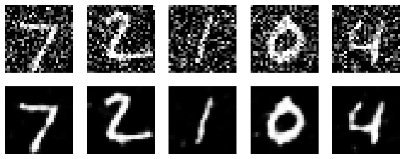
Challenge: Complete the training of the autoencoder network and, referring to the experimental content, use the first 5 test samples to compare the effects before and after denoising.
## 补充代码 ###
Solution to Exercise 67.2
X_train_noisy = X_train_noisy.reshape(-1, 28, 28, 1)
X_train = X_train.reshape(-1, 28, 28, 1)
model.fit(X_train_noisy, X_train, batch_size=64, epochs=3)
from matplotlib import pyplot as plt
%matplotlib inline

n = 5
decoded_code = model.predict(
    X_test_noisy[:n].reshape(-1, 28, 28, 1))  # Autoencoder inference
plt.figure(figsize=(10, 6))
for i in range(n):
    # Output the original test sample image
    ax = plt.subplot(3, n, i+1)
    plt.imshow(X_test_noisy[i].reshape(28, 28), cmap='gray')
    ax.get_xaxis().set_visible(False)
    ax.get_yaxis().set_visible(False)

    # Output the image after denoising by the autoencoder
    ax = plt.subplot(3, n, i+n+1)
    plt.imshow(decoded_code[i].reshape(28, 28), cmap='gray')
    ax.get_xaxis().set_visible(False)
    ax.get_yaxis().set_visible(False)
Expected output: