Pro Membership

Pro Membership is a membership plan created by the author to maintain and update this tutorial. You can get more benefits and services, click to view details.

38. Time Series Data Modeling and Analysis

38.1. Introduction

Previously, we have learned some methods and techniques for time series processing using Pandas. In this experiment, we will guide you to learn about relevant models for time series data analysis and use some well-known tools to complete time series modeling and analysis.

38.2. Key Points

• Characteristics and Classification of Time Series Data

• Descriptive Time Series Analysis

• Statistical Time Series Analysis

• Stationarity Test of Time Series

• Autocorrelation Plot and Partial Autocorrelation Plot

• Pure Randomness Test

• Introduction and Modeling of ARMA

• Differencing Operation

• Introduction and Modeling of ARIMA

Previously, we learned the relevant operations for processing time series data using Pandas. In fact, when we face time series data, we want to analyze some patterns from it and predict the possible changes in values in the future. For example, we may need to analyze the future stock price trends of a company from stock data, obtain the weather information at a certain future moment from meteorological data, and discover the possible upcoming peaks from access log data.

After we have learned machine learning modeling, you may think of applying it to the time series modeling process. For example, for a time series change graph with time on the horizontal axis and values on the vertical axis. Can a regression model be introduced for prediction?

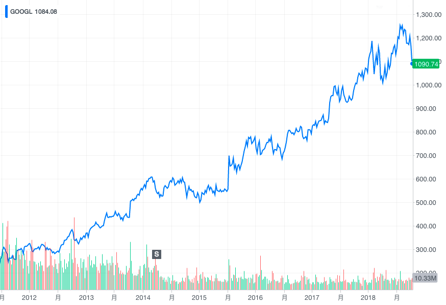
The above figure presents the stock price change curve. Can we convert the year into a serial number and thus introduce regression analysis to obtain future prediction results? The answer is definitely “yes”, because there is no theoretical obstacle to achieving it by regression means. However, this is only a discussion about the application of the method. As for the effect of regression prediction, we have no idea.

In regression prediction, we have given a very classic example, which is housing price prediction. Generally, the price of a house is positively correlated with its area. That is to say, if we build a regression model with these two variables, generally, the larger the area of the house, the higher the price. Then, if we change the data to temperature change data. During the transition from spring to summer, the temperature will gradually increase with time, but this relationship will not continue like that of housing prices. Because the change in temperature will become flat after a certain time and fluctuate within a certain range. At this time, if we apply a regression model to predict the temperature, it cannot accurately reflect the current situation.

38.3. Characteristics and Classification of Time Series Data

To analyze time data and discover patterns, we first need to understand the characteristics of time series data:

• Time series data depends on time, but it is not necessarily a strict function of time.

• The values of time series data at each moment have a certain degree of randomness and cannot be predicted completely accurately using historical values.

Meanwhile:

• The numerical values of time series data at successive moments (but not necessarily adjacent moments) often have correlations.

• Overall, time series often exhibit some kind of trend or periodic variation.

After understanding the above four characteristics, you may feel that if you directly apply regression analysis in machine learning to time series prediction, the results may not be very satisfactory.

In the study of time series data, we usually subdivide it into the following different types according to different dimensions:

• Classification by research object: univariate time series and multivariate time series.

• Classification by time parameter: discrete time series and continuous time series.

• Classification by statistical characteristics: stationary time series and non-stationary time series.

• Classification by distribution law: Gaussian time series and non-Gaussian time series.

38.4. Descriptive Time Series Analysis

Descriptive time series analysis, also known as deterministic time series analysis, mainly seeks the development laws contained in the series through intuitive data comparison or plotting observations. This method is simple and direct, so it is generally the first step in time series analysis.

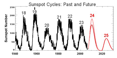
For example, in 1844, the German astronomer Heinrich Schwabe reported the periodic variation law of sunspot numbers in Astronomische Nachrichten. Through systematic continuous observations, he found that the eruptions of sunspots showed a periodic variation with a period of about 11 years.

38.5. Statistical Time Series Analysis

Although the descriptive analysis method is intuitive, it has high requirements for data. It is necessary to ensure that the data distribution shows a certain regularity in order to obtain credible conclusions from it. However, in many cases, the time series data we encounter shows obvious randomness, making it difficult to accurately predict its trend and change law.

于是，统计时序分析相关方法开始出现，人们尝试利用数理统计学相关的原理和方法来分析时间序列。 As a result, methods related to statistical time series analysis began to emerge, and people tried to use the principles and methods of mathematical statistics to analyze time series.

In statistical time series analysis, it is generally subdivided into two different types of analysis methods, namely: frequency domain analysis and time domain analysis.

Frequency domain analysis, simply put, is that we assume that any trendless time series can be decomposed into periodic fluctuations of several different frequencies. Early frequency domain analysis methods used Fourier analysis to reveal the laws of time series from the perspective of frequency. Later, it used the Fourier transform to approximate a function with the sum of sine and cosine terms. Then, with the introduction of the maximum entropy spectral estimation theory, frequency domain analysis entered the stage of modern spectral analysis. Due to the fact that spectral analysis relies on a strong mathematical background and is not conducive to intuitive interpretation, this method has great limitations, and we will not introduce it in too much detail.

Different from frequency domain analysis, time domain analysis methods are much more widely applied. The principle of time domain analysis mainly refers to the inertia in the process of event development. Statistically described through inertia, it is the correlation existing between time series values, and this kind of correlation usually has a certain statistical law. The purpose of time domain analysis is to find out the statistical law of the correlation between time series values, fit an appropriate mathematical model to describe this law, and then use this fitted model to predict the future trend of the series.

The emergence of time domain analysis methods can be traced back to the autoregressive AR model that appeared in 1927. Soon after, Sir Walker, a British mathematician and astronomer, used the moving average MA model and the autoregressive moving average ARMA model when analyzing the atmospheric laws in India. These models laid the foundation for time series time domain analysis methods, and the ARMA model among them has also been widely applied. Later, American statistician Box and British statistician Jenkins systematically expounded the principles and methods of identifying, estimating, testing, and predicting the autoregressive integrated moving average ARIMA model. This knowledge is now known as the classical time series analysis method and is the core content of time domain analysis methods.

Among them, the ARMA model is usually used in the analysis process of stationary time series, while the ARIMA model is widely applied in the stochastic analysis process of non-stationary series.

{note}
Note: In the following content, a large number of statistical theories and principles in econometrics will be involved. We will not derive and calculate complex theories, but directly present the concepts and tell you their uses and applications.

38.6. Stationary Time Series Test

What is a stationary time series? This requires us to define it from the perspective of probability and statistics. Generally speaking, there are two definitions of stationary time series, namely: strictly stationary time series and weakly stationary time series. Among them, strict stationarity requires that all statistical properties of the series do not change over time. Weak stationarity believes that as long as the second moment of the series is stationary, it means the series is stable. Obviously, strict stationarity has stricter conditions than weak stationarity. Strict stationarity is a requirement for the joint distribution of the series to ensure that all statistical characteristics of the series are the same.

Regarding the test for the stationarity of a series, there are generally two methods, namely: graphical test and hypothesis test. The graphical test makes a judgment based on the characteristics shown in the time series plot and the autocorrelation plot, and is widely used because of its simple operation. Simply put, if a time series plot shows an obvious increasing and decreasing trend, then it must be non-stationary.

Next, we present the curve graph of the population quantity change in China, which is a time series composed of years. We call this set of data series1.

wget -nc https://cdn.aibydoing.com/aibydoing/files/total-population.csv

import pandas as pd
from matplotlib import pyplot as plt

%matplotlib inline

series1 = pd.read_csv("total-population.csv", index_col=0)
series1.plot(figsize=(9, 6))

<Axes: xlabel='year'>

It can be seen that series1 shows an obvious increasing trend, so it must not be a stationary time series.

Next, let’s take a look at another time series data. Here we use NumPy to generate a random series and call it series2.

import numpy as np

np.random.seed(10)  # 随机数种子
series2 = np.random.rand(1000)  # 生成随机序列
plt.plot(series2)  # 绘图
plt.ylim(5, -5)

(5.0, -5.0)

It can be seen that the sequence of series2 fluctuates randomly above and below a certain value, without obvious trends and periodicity. Generally speaking, we would consider this type of sequence to be stationary.

However, for the stationary curve graph shown above, we generally need to further confirm it through the autocorrelation graph.

38.7. Autocorrelation Graph

Autocorrelation, also known as serial correlation, is a concept in statistics. Correlation is actually the strength of the relationship between variables, and here we will use the Pearson correlation coefficient learned before for testing.

In a time series, when we calculate the correlation of time series observations using previous time steps. Since the correlation of the time series is calculated with values of the same series as before, it is called autocorrelation. Among them, the autocorrelation function ACF is used to measure the correlation between sequence values that are \(k\) time intervals (delay periods) apart when the delay in the time series is \(k\), and the resulting graph is called the autocorrelation graph.

The calculation diagram of ACF is as follows. The original sequence calculates the correlation coefficient with the original sequence after a delay of \(k\) time intervals (the green part).

In Python, we can use the plot_acf() function in the statsmodels statistical calculation library to calculate and plot the autocorrelation graph, or we can also use the autocorrelation_plot() method provided by Pandas to plot it.

from statsmodels.graphics.tsaplots import plot_acf
from pandas.plotting import autocorrelation_plot

fig, axes = plt.subplots(ncols=2, nrows=1, figsize=(12, 4))

plot_acf(series1, ax=axes[0])
autocorrelation_plot(series1, ax=axes[1])

<Axes: xlabel='Lag', ylabel='Autocorrelation'>

from statsmodels.graphics.tsaplots import plot_acf
from pandas.plotting import autocorrelation_plot

fig, axes = plt.subplots(ncols=2, nrows=1, figsize=(12, 4))

plot_acf(series1, ax=axes[0])
autocorrelation_plot(series1, ax=axes[1])

<Axes: xlabel='Lag', ylabel='Autocorrelation'>

In the above figure, we plot the autocorrelation graph of series1. Among them, the vertical axis value of the ACF graph represents the correlation, and the Pearson correlation coefficient corresponds to values between -1 and 1.

Next, we also plot the autocorrelation graph of series2.

fig, axes = plt.subplots(ncols=2, nrows=1, figsize=(12, 4))

plot_acf(series2, ax=axes[0])
autocorrelation_plot(series2, ax=axes[1])

<Axes: xlabel='Lag', ylabel='Autocorrelation'>

So, how can we judge the stationarity of a time series through the autocorrelation graph? As shown in the autocorrelation graphs corresponding to series1 and series2, stationary series usually have short-term correlations. This property is described by the autocorrelation coefficient that as the lag \(k\) increases, the autocorrelation coefficient of a stationary series will quickly decay to zero. On the contrary, the autocorrelation coefficient of a non-stationary series usually decays to zero at a relatively slow speed, which is the criterion for us to judge stationarity using the autocorrelation graph. Therefore, the series corresponding to series2 is a stationary time series, while series1 is a non-stationary time series.

Meanwhile, since the autocorrelation coefficients of the series shown in the autocorrelation graph corresponding to series2 are always small and fluctuate around 0, we would consider this to be a stationary time series with a very strong randomness.

38.8. Pure Randomness Test

Generally speaking, after obtaining a time series, we will conduct a stationarity test on it. If the series is stationary, then mature modeling methods such as ARMA can be applied to complete the analysis. However, not all stationary series are worth modeling. For example, the above series2 series, although stationary, has too strong randomness. Generally speaking, a pure random series has no analytical value.

So, a new problem arises: how to determine whether a stationary series is random? This is where the pure randomness test comes into play. In the process of the pure randomness test, generally two statistics are involved, namely: the Q statistic and the LB statistic (Ljung-Box). However, since the LB statistic is a correction of the Q statistic, the Q statistic commonly referred to in the industry is actually the LB statistic.

In Python, we can use the acorr_ljungbox() function in the statsmodels statistical calculation library to calculate the LB statistic. This function will return the LB statistic and the P-value of the LB statistic by default. If the P-value of the LB statistic is less than 0.05, we consider this series to be a non-random series; otherwise, it is a random series.

from statsmodels.stats.diagnostic import acorr_ljungbox

P2 = acorr_ljungbox(series2).lb_pvalue
plt.plot(P2)

[<matplotlib.lines.Line2D at 0x13544e890>]

As shown above, the P-value corresponding to the LB statistic of series2 is much larger than 0.05. Therefore, it can be determined that it is a random series and there is no need for further analysis.

Next, let’s take a look at the parameters of a non-random stationary time series. The experiment gives the sunspot statistical data series3 from 1820 to 1870, which is plotted as follows:

wget -nc https://cdn.aibydoing.com/aibydoing/files/sunspot.csv

series3 = pd.read_csv("sunspot.csv", index_col=0)
series3.index = pd.period_range("1820", "1869", freq="Y")  # 将索引转换为时间
series3.plot(figsize=(9, 6))

<Axes: >

Then, perform the first step of processing the time series: the stationarity test. The autocorrelation plot is drawn as follows:

fig, axes = plt.subplots(ncols=2, nrows=1, figsize=(12, 4))

plot_acf(series3, ax=axes[0])
autocorrelation_plot(series3, ax=axes[1])

<Axes: xlabel='Lag', ylabel='Autocorrelation'>

It can be seen that in the autocorrelation plot, as the number of lags increases, it approaches 0. However, it does not fluctuate around 0 like the random series above, and then shows periodic changes later. Therefore, it can be judged as a periodically varying stationary series.

Next, we conduct the pure randomness test. Calculate the LB statistic and the corresponding P-value of the series as the number of lags increases, and plot the image of the P-value change.

P3 = acorr_ljungbox(series3).lb_pvalue
plt.plot(P3)

[<matplotlib.lines.Line2D at 0x13567eaa0>]

As shown in the figure above, the P-value is much less than 0.05 (note the unit of the vertical axis), indicating that the series is a non-purely random series.

Above, we introduced the preprocessing steps for time series, namely: stationarity test and pure randomness test, and these two steps are often important steps before time series analysis and modeling. Next, we will formally introduce the time series modeling process.

38.9. Introduction and Modeling of ARMA

The full name of the ARMA model is the autoregressive moving average model, which is currently the most commonly used model for fitting stationary sequences. The ARMA model can generally be further divided into three categories: the AR autoregressive model, the MA moving average model, and the ARMA model.

The AR model is very simple, and its idea comes from linear regression. That is, assume that the sequence contains a linear relationship, and then use the sequence of \(x_{1}\) to \(x_{t - 1}\) to predict \(x_{t}\). Among them, the formula for the p-order AR model is:

\[X_{t}=c+\sum _{{i=1}}^{p}\varphi _{i}X_{{t-i}}+\varepsilon _{t}\]

Among them, \({c}\) is the constant term. \(\varepsilon _{t}\) is assumed to be a random error value with an average of 0 and a standard deviation of \({\sigma}\). \({\sigma}\) is assumed to be constant for any \({t}\). \(p\) represents the number of lag periods.

If the stochastic process \(x_t\) is a weighted average of the current and the past \(q\) - period stochastic processes \(ε_t, ε_{t - 1},..., ε_{t−q}\), then the formula for the \(q\) - order MA model is:

\[{x_{t}=\varepsilon _{t} + \theta _{1}\varepsilon _{t-1} + \theta _{2}\varepsilon _{t-2} + \cdots + \theta _{q}\varepsilon _{t-q}}\]

Among them, \(θ_1,..., θ_q\) are parameters, and \(ε_t, ε_{t - 1},..., ε_{t−q}\) are all white noises.

Here, we do not elaborate on the proof processes of the AR and MA models, so the above formulas may be very difficult to understand. Since the derivation process is too complex, if you are interested, you need to set aside other time for self - study.

The ARMA model is generally denoted as: \(ARMA(p,q)\), which is a combination of the \(p\) - order AR and \(q\) - order MA models. In Python, we can use the tsa.ARMA class in the statsmodels statistical computing library to complete ARMA modeling and prediction.

Next, taking the sunspot dataset series3 as an example, we complete an ARMA modeling process. Before modeling, we first need to determine the values of \(p\) and \(q\). Generally speaking, there are three methods to determine their values, namely AIC (Akaike Information Criterion), BIC (Bayesian Information Criterion), and HQIC (Hannan - Quinn Criterion).

The calculation methods of the three metrics are as follows:

import warnings
from statsmodels.tsa.stattools import arma_order_select_ic

train_data = series3[:-10]  # 80% 训练
test_data = series3[-10:]

warnings.filterwarnings("ignore")
arma_order_select_ic(train_data, ic="aic")["aic_min_order"]  # AIC

(2, 1)

arma_order_select_ic(train_data, ic="bic")["bic_min_order"]  # BIC

(2, 0)

arma_order_select_ic(train_data, ic="hqic")["hqic_min_order"]  # HQIC

(2, 1)

The different calculation methods lead to different results. You can try them all to see the results. Since the results of AIC and HQIC are the same, we will use \(p = 2\) and \(q = 1\) as suggested by the AIC method. Next, we start to define and build the ARMA model.

from statsmodels.tsa.arima.model import ARIMA

arma = ARIMA(train_data, order=(2, 0, 1)).fit()  # 定义并训练模型

arma.forecast(steps=10).values

array([111.37037427, 100.57459254,  75.88578412,  51.33635506,
        35.73963142,  31.42983122,  35.80573077,  44.08789217,
        51.84682424,  56.47354706])

Next, we output the test results and compare them with the actual results.

plt.plot(arma.forecast(steps=10).values, ".-", label="predict")  # 输出后续 10 个预测结果
plt.plot(test_data.values, ".-", label="real")
plt.legend()

<matplotlib.legend.Legend at 0x1351449d0>

It can be seen that the prediction results can still accurately reflect the data trend. Regarding the evaluation of the ARMA model, it will not be elaborated here, because it is all continuous numerical prediction, and the relevant methods learned in regression analysis can be used for evaluation. For example, calculate metrics such as MSE.

Finally, we summarize the ARMA modeling steps as follows:

Obtain the sequence → Conduct the stationarity test → Conduct the pure randomness test → Estimate the \(p\) and \(q\) parameters → ARMA modeling → Model evaluation

Above, in the process of modeling time series through ARMA, we first need to make the series meet the requirement of “stationarity”. So, for non-stationary series, such as the series1 series of population changes at the beginning, what should we do if we want to analyze it?

At this time, if we can find a way to make the series more stationary, then we can apply ARMA for calculation. And here we need to learn a method to make the series stationary: differencing.

38.10. Differencing Operation

Differencing operation is actually a method to extract deterministic information from a series, and it is also a very basic mathematical analysis tool. Below, we review the method and formula for differencing calculation.

If we perform a subtraction operation on the adjacent values (with a lag of 1 period) of two series, we can denote \(\nabla x_t\) as the first-order difference of \(x_t\), and the formula is as follows:

\[\nabla x_t = x_t - x_{t-1}\]

At this time, if we perform another first-order differencing operation on the series after the first-order differencing, we can denote \(\nabla^2 x_t\) as the second-order difference of \(x_t\), and the formula is as follows:

\[\nabla^2 x_t = \nabla x_t - \nabla x_{t - 1}\]

Then, by analogy, if we perform another first-order differencing operation on the series after the \((p - 1)\)-order differencing, we can denote \(\nabla^p x_t\) as the \(p\)-order difference of \(x_t\), and the formula is as follows:

\[\nabla^p x_t = \nabla^{p - 1} x_t - \nabla^{p - 1} x_{t - 1}\]

In addition, if we perform a subtraction operation between two sequence values with a delay of \(k\) periods, it is called a \(k\)-step differencing operation. Denote \(\nabla_k x_t\) as the \(k\)-step difference of \(x_t\), and the formula is as follows:

\[\nabla_k x_t = x_t - x_{t - k}\]

Next, we use Pandas to perform a first-order differencing operation on the series1 sequence, plot the results, and simultaneously conduct stationarity and pure randomness tests on the differenced data.

fig, axes = plt.subplots(ncols=3, nrows=1, figsize=(15, 3))

diff1 = series1.diff().dropna()  # 1 阶差分

axes[0].plot(diff1)  # 绘图
autocorrelation_plot(diff1, ax=axes[1])  # 平稳性检验
axes[2].plot(acorr_ljungbox(diff1).lb_pvalue)  # 纯随机检验

[<matplotlib.lines.Line2D at 0x1365a26b0>]

Try the first-order two-step differencing:

fig, axes = plt.subplots(ncols=3, nrows=1, figsize=(15, 3))

diff1 = series1.diff(periods=2).dropna()  # 1 阶 2 步差分

axes[0].plot(diff1)  # 绘图
autocorrelation_plot(diff1, ax=axes[1])  # 平稳性检验
axes[2].plot(acorr_ljungbox(diff1).lb_pvalue)  # 纯随机检验

[<matplotlib.lines.Line2D at 0x136702b90>]

It seems that adjusting the step size of differencing cannot effectively improve stability. Next, we perform second-order differencing:

fig, axes = plt.subplots(ncols=3, nrows=1, figsize=(15, 3))

diff2 = series1.diff().diff().dropna()  # 2 阶差分

axes[0].plot(diff2)  # 绘图
autocorrelation_plot(diff2, ax=axes[1])  # 平稳性检验
axes[2].plot(acorr_ljungbox(diff2).lb_pvalue)  # 纯随机检验

[<matplotlib.lines.Line2D at 0x13714c580>]

As mentioned above, the second-order differencing makes the data much more stationary, so we choose \(d = 2\).

Generally, the order of differencing should not be too large. The reason is that differencing is actually a process of information extraction and processing, and each differencing will cause information loss. Excessive differencing will lead to the loss of effective information and reduce the accuracy. Generally, a linear change can be made stationary through one-time differencing, and a non-linear trend can also be made stationary through two or three times of differencing. Generally, the number of differencing times does not exceed two times.

38.11. Introduction and Modeling of ARIMA

As mentioned above, the ARIMA model is suitable for modeling and analyzing non-stationary sequences. You may have noticed that ARIMA has one more letter ‘I’ than ARMA. In fact, this ‘I’ represents differencing. At the same time, compared with the \(p\) and \(q\) parameters in the ARMA model, ARIMA has one more parameter, which is the order of differencing \(d\) used to make the non-stationary sequence become a stationary sequence. Therefore, the ARIMA model is usually denoted as: \(ARIMA(p, d, q)\).

Next, we use the differenced data to determine the \(p\) and \(q\) parameters. This step is similar to ARMA modeling. Here we use the AIC solution results to determine the parameters. Of course, we can also use the other two methods.

train_data = series1[:-40]  # 约 80% 训练
test_data = series1[-40:]

arma_order_select_ic(train_data.diff().dropna(), ic="aic")["aic_min_order"]  # AIC

(3, 0)

Note that we will determine the \(p\) and \(q\) parameters based on the differencing results. According to the value of AIC, we determine that \(p = 3\) and \(q = 0\).

from statsmodels.tsa.arima.model import ARIMA

arima = ARIMA(train_data, order=(3, 2, 0)).fit()  # 定义并训练模型

Similarly, the test results are output here and compared with the actual results.

plt.plot(arima.forecast(steps=40).values, ".-", label="predict")  # 输出后续 40 个预测结果
plt.plot(test_data.values, ".-", label="real")
plt.legend()

<matplotlib.legend.Legend at 0x1371fa9b0>

As can be seen from the figure, the prediction results basically conform to the trend of the actual data. Finally, we summarize the general process of time series analysis and modeling as follows:

38.12. Summary

In this experiment, we learned some theoretical methods related to time series analysis and modeling, and studied the modeling ideas of using ARMA and ARIMA for stationary and non-stationary time series. At the same time, we completed the modeling analysis process by applying the well-known statsmodels library in Python.

The experiment has sorted out the process of time series modeling, but has not conducted in-depth discussions and derivations on the statistical theories involved. The reason is that the amount of theoretical knowledge involved has far exceeded the expectations of the course. If you are very interested in the time series analysis process, you are welcome to purchase and read Applied Time Series Analysis published by Renmin University of China Press. Renmin University of China, as the most famous institution in the domestic statistics major, also uses this book for undergraduate teaching.

Related Links

• Wang Yan, Applied Time Series Analysis

---

○ Sharethis article link to your social media, blog, forum, etc. More external links will increase the search engine ranking of this site.

If you find this content helpful, you can buy me a coffee

Previous

37. Stock Time Series Data Processing

Next

39. Agricultural Production Index Modeling Analysis