16. Gaussian Distribution Function Implementation and Plotting#
16.1. Introduction#
The Gaussian distribution was mentioned in the Naive Bayes experiment. In this challenge, the Gaussian distribution function is implemented in Python, and the Gaussian distribution images under different parameters are plotted using Matplotlib.
16.2. Key Points#
Gaussian distribution formula
Gaussian distribution function
16.3. Gaussian Distribution Formula#
In the Naive Bayes experiment, we know that according to the type of feature data, the Naive Bayes model can be divided when calculating the prior probability, and it can be divided into: multinomial model, Bernoulli model, and Gaussian model. In the previous experiment, we used the multinomial model to complete it.
Most of the time, when our features are continuous variables, the performance of using the multinomial model is not good. Therefore, we usually adopt the Gaussian model to process continuous variables, and the Gaussian model actually assumes that the feature data of continuous variables follows a Gaussian distribution. Among them, the expression of the Gaussian distribution function is:
Among them, \(\mu\) is the mean value and \(\sigma\) is the standard deviation.
Exercise 16.1
Challenge: Refer to the Gaussian distribution formula and implement the Gaussian distribution function using Python.
"""实现高斯分布函数
"""
import numpy as np


def Gaussian(x, u, d):
    """
    参数:
    x -- 变量
    u -- 均值
    d -- 标准差

    返回:
    p -- 高斯分布值
    """
    ### 代码开始 ### (≈ 3~5 行代码)
    p = None

    return p
    ### 代码结束 ###
Solution to Exercise 16.1
"""Implement the Gaussian distribution function
"""
import numpy as np

def Gaussian(x, u, d):
    """
    Parameters:
    x -- variable
    u -- mean value
    d -- standard deviation

    Returns:
    p -- Gaussian distribution value
    """
    ### START CODE HERE ### (≈ 3~5 lines of code)
    d_2 = d * d * 2
    zhishu = -(np.square(x - u) / d_2)
    exp = np.exp(zhishu)
    pi = np.pi
    xishu = 1 / (np.sqrt(2 * pi) * d)
    p = xishu * exp
    return p
    ### END CODE HERE ###
Run the test
x = np.linspace(-5, 5, 100)
u = 3.2
d = 5.5
g = Gaussian(x, u, d)

len(g), g[10]
Expected output
(100,
                      0.030864654760573856)
After implementing the Gaussian distribution function, we can use Matplotlib to plot the Gaussian distribution images with different parameters.
Exercise 16.2
Challenge: Plot Gaussian distribution images with specified parameters.
Requirements:
-
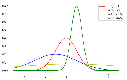
Plot 4 sets of Gaussian distribution line images with \(\mu\) and \(\sigma\) being
(0,
                              1),
                              (-1,
                              2),
                              (1,
                              0.5),
                              (0.5,
                              5)
respectively. -
The line colors of the 4 sets of Gaussian distribution images are red, blue, green, and yellow respectively.
-
Plot a legend and present it in the style of \(u = \sigma\).
from matplotlib import pyplot as plt

%matplotlib inline

## 代码开始 ### (≈ 5~10 行代码)

## 代码结束 ###
Solution to Exercise 16.2
from matplotlib import pyplot as plt
%matplotlib inline

### Code start ### (≈ 5 - 10 lines of code)
y_1 = Gaussian(x, 0, 1)
y_2 = Gaussian(x, -1, 2)
y_3 = Gaussian(x, 1, 0.5)
y_4 = Gaussian(x, 0.5, 5)

plt.figure(figsize=(8,5))
plt.plot(x, y_1, c='r', label="u=0, d=1")
plt.plot(x, y_2, c='b', label="u=-1, d=2")
plt.plot(x, y_3, c='g', label="u=1, d=0.5")
plt.plot(x, y_4, c='y', label="u=0.5, d=5")
plt.legend()
### Code end ###
Expected output