Pro Membership

Pro Membership is a membership plan created by the author to maintain and update this tutorial. You can get more benefits and services, click to view details.

90. Basic Probability Theory and Statistics in Python

90.1. Introduction

Probability theory is a mathematical framework for representing statements of uncertainty. The design of many machine learning algorithms relies on probabilistic assumptions about the data. Similarly, we can also use knowledge of probability and statistics to theoretically analyze the behavior of the AI systems we propose. This experiment mainly describes the probability theory and statistical learning methods commonly used in machine learning.

90.2. Key Points

• Probability formulas

• Random variables

• Probability distributions

• Mathematical expectations

• Variance, standard deviation, and covariance

• Hypothesis testing

Probability theory is a mathematical framework for representing statements of uncertainty. The design of many machine learning algorithms relies on probabilistic assumptions about the data. Similarly, we can also use knowledge of probability and statistics to theoretically analyze the behavior of the AI systems we propose. Next, let’s introduce several of the most important probability formulas in probability theory.

90.3. Conditional Probability

Conditional probability is the probability under a certain condition. For example, when event \(A\) occurs, the probability that event \(B\) occurs can be called conditional probability, denoted as \(P(B|A)\). Another example is that given the condition \(x = a\), the probability that \(y = b\) is conditional probability, denoted as \(P(y = b|x = a)\). The condition is recorded on the right side of the vertical bar in the parentheses, and the result is recorded on the left side.

The calculation formula for the conditional probability \(P(B|A)\) is as follows:

\[P(B|A)=\frac{P(AB)}{P(A)}\]

For example, there are 100 old and new table tennis balls mixed in a box, and these table tennis balls are of two colors, red and yellow. The classification is as follows:

	Yellow	White
New	40	30
Old	20	10

If I take out a ball from the box and it is known that the ball is yellow, then what is the probability that the ball is new?

We can see from the above table that the probability that this yellow ball is new is \(P = \frac{40}{60}\) (since it is already known that the ball is yellow, so the denominator is 60).

Of course, we can also use the method of conditional probability mentioned above:

Let event A = {randomly pick a ball from the box and the ball is yellow}, then according to the above table, \(P(A)=\frac{20 + 40}{100}=\frac{60}{100}\).

Let event B = {randomly pick a ball from the box and the ball is new}, then according to the above table, the probability that the ball taken out is a new yellow ball is: \(P(AB)=\frac{40}{100}\).

Then the probability that a ball is new given that it is yellow is as follows:

\[P(B|A)=\frac{P(AB)}{P(A)}=\frac{{40}/{100}}{{60}/{100}}=\frac{40}{60}\]

Note that here \(P(AB)\neq P(A)\times P(B)\) because events A and B are not independent.

90.4. Total Probability Theorem

Definition: Let \(A_1,A_2,...A_n\) be a sequence of mutually exclusive events such that \(A_1 \cup A_2 \cup,... \cup A_n=\Omega\). Then for any event B, the following relationship holds:

\[P(B)=\sum_{i=1}^nP(A_i)P(B|A_i) \]

The Total Probability Theorem can be explained by the following figure:

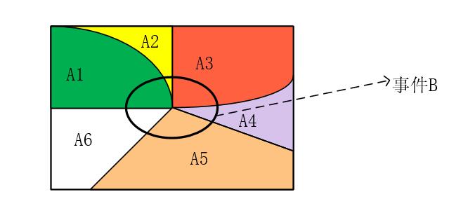
When it is very difficult to directly obtain \(P(B)\), we can divide event \(B\) into multiple parts: $\( P(B) = P(A_1B)+ P(A_2B)+P(A_3B)+P(A_4B)+P(A_5B)\)$

Then, according to the conditional probability formula, transform the above formula:

\[P(B)=\sum_{i=1}^nP(A_iB) =\sum_{i=1}^nP(A_i)P(B|A_i) \]

This is the origin of the total probability formula. The main idea of this formula is that when it is difficult to calculate \(P(A)\), we can decompose event \(A\) into several small events, calculate the probabilities of the small events, and then add them up to obtain the probability of the large event.

Take a simple example. Suppose there are four machine tools, namely A, B, C, and D, used in a workshop. The defective rates of each machine tool are 5%, 4%, 3%, and 3.5% respectively, and their respective products account for 20%, 35%, 25%, and 20% of the total output. Now mix them together and ask about the probability of randomly taking out a defective product.

Idea: According to the problem description, we can know that:

• The probability \(P(A_i)\) that a certain product comes from a certain machine tool is \([20\%, 35\%, 25\%, 20\%]\) (estimating the probability using the usage proportion).

• The defective rate \(P(B|A_i)=[5\%, 4\%, 3\%, 3.5\%]\) (this defective rate is the defective rate under each machine tool, with the denominator being the number of products of each machine tool respectively).

And what we need to find now is \(P(B)\), that is, the defective rate with the denominator being the total number of products. According to the total probability formula, we can use vector multiplication to obtain the defective rate of this product:

import numpy as np

# 将百分数转为小数
pa = np.array([20.0, 35, 25, 20])*0.01
pb_A = np.array([5.0, 4, 3, 3.5])*0.01
# 利用全概率公式计算次品率:先相乘再求和
pb = np.sum(np.multiply(pa, pb_A))

print("总次品率为：{}%".format(pb*100))

总次品率为：3.85%

90.5. Bayes’ Theorem

Definition: Let \(A_1, A_2, \ldots, A_n\) be a sequence of mutually exclusive events such that \(A_1 \cup A_2 \cup \ldots \cup A_n = \Omega\). If event B has occurred now, the probability that \(A_i\) occurs:

\[P(A_i|B)=\frac{P(AB_i)}{P(B)}=\frac{P(A_i)P(B|A_i)}{P(B)}\]

The above formula is the derivation of Bayes’ theorem. In fact, whether it is the derivation of the total probability formula or Bayes’ theorem, their core is to use the conditional probability formula.

Differences between Bayes’ theorem and the total probability formula: Suppose there are several ways to achieve the same goal, and the probabilities of achieving the goal by each way are different. The total probability formula is used to calculate the probability value of finally achieving the goal (regardless of which way is used). While Bayes’ theorem calculates the probability of using each way given that the goal has been achieved.

Still taking the example of machining products by machine tools above, let the event that the extracted product is defective be event B, and the event that the \(i\)-th machine tool produces products be event \(A_i\), with other data remaining unchanged.

Suppose all the products are still mixed together and then one product is randomly selected. It is found that this product is defective. What is the probability \(P(A_i|B)\) that this product comes from each machine tool?

According to the problem, what we need to find is \(P(A_i|B)\). Then, using Bayes’ theorem, we can calculate:

# 根据贝叶斯公式，计算来自每个机床的概率
# 这里的 pb 可以通过全概率公式进行计算
pA_b = (pa*pb_A) / pb

for i in range(4):
    print("该产品来自第 {} 个机床的概率：{}".format(i+1, pA_b[i]))

该产品来自第 1 个机床的概率：0.25974025974025977
该产品来自第 2 个机床的概率：0.3636363636363637
该产品来自第 3 个机床的概率：0.1948051948051948
该产品来自第 4 个机床的概率：0.18181818181818185

90.6. Probability Distribution

90.7. Data Types

In programming, we often need some random values (such as when simulating coin flips). We call the variables that store these random values random variables.

Random variables can be divided into two types according to the range of values they generate:

• Discrete random variable: If the random variable \(X\) can only take a finite number or at most a countable number of values, then \(X\) is called a discrete random variable. For example, a random variable taking values from the set \(\{0, 1\}\) is a discrete variable (only two values exist).

• Continuous random variable: If all possible values of the random variable \(X\) cannot be listed one by one, but take any random value at any point within a certain interval on the number line, then \(X\) is a continuous random variable. For example, a random variable taking values in the interval \((0, 1]\) is a continuous variable (there are infinitely many points between 0 and 1).

Regardless of the type of random variable, the principle of its generation is to assign a probability to each possible value within its range, and then randomly assign a value to the variable according to the probability.

The probability functions that describe all possible values can be further divided according to the variable type into:

• Probability mass function: The probability function that describes the possible values of a discrete variable.

• Probability density function: The probability distribution function that describes a continuous variable.

Probability distribution refers to the probability law of a random variable. Simply put, the probability distribution describes the probability corresponding to each possible value of the random variable. When simulating data, we assign different values to the data according to different probabilities. Next, let’s introduce in detail the common discrete probability distributions and continuous probability distribution functions.

Note that for beginners, we don’t have to memorize the specific forms of each function. What we should understand more is the characteristics and applicable ranges of each distribution function.

90.8. Discrete Probability Distributions

In life, the results of many events often have only two outcomes. For example: the result of flipping a coin (heads up or tails up), inspecting the quality of a product (qualified or unqualified), buying a lottery ticket (winning or not winning). All of the above events can be called Bernoulli trials.

A Bernoulli trial is actually a single random trial with only two possible outcomes, 0 or 1, and was proposed by the scientist Bernoulli. The data distribution generated by a Bernoulli trial is the Bernoulli distribution.

Bernoulli Distribution: That is, the most common 0-1 distribution. The variable following this distribution has only two possible values, 0 and 1. The probability mass function of this distribution is as follows:

\[ P(x) = \begin{cases} \lambda & \text{if } x = 1 \cr 1 - \lambda & \text{if } x = 0 \end{cases} \]

Among them, the possible values of \(x\) are \(\{0, 1\}\). \(\lambda\) is the probability of a successful result and can be any value in \([0, 1]\). \(P(x)\) represents the probability that the result is \(x\).

We can generate random numbers based on the probabilities corresponding to each \(x\). As follows:

def Bernoulli(lambd_a):
    p = np.random.rand()
    # 表示返回 1 的概率 为 lambda
    if(p < lambd_a):
        return 1
    else:
        return 0

We can use the above function to simulate coin - tossing. Suppose we toss a coin 5 times:

for i in range(5):
    print("第{}次实验结果：".format(i+1))
    result = Bernoulli(0.5)  # 每面的结果概率相同
    if(result == 1):
        print("正面")
    else:
        print("反面")

第1次实验结果：
正面
第2次实验结果：
反面
第3次实验结果：
正面
第4次实验结果：
反面
第5次实验结果：
反面

Binomial Distribution: The probability distribution of the number of times the result is 1 after \(n\) Bernoulli trials, that is, the probability distribution of the number of successful trials, where the probability of success in each trial is \(p\).

If the probability of success in each experiment is \(p\), and then we conduct \(n\) trials, what is the probability of a total of \(x\) successes? We can obtain the following formula through permutations and combinations:

\[P(x) =C_n^xp^x(1-p)^{n-x} =\frac{n!}{x!(n-x)!}p^x(1-p)^{n-x}\]

Among them, \(C_n^x\) is a permutation and combination, representing selecting \(x\) experiments out of \(n\) trials. \(p^x\) represents the probability that all the selected experiments are successful. \((1 - p)^{n - x}\) represents the probability that all the unselected experiments are failed.

In fact, the above function is the probability mass function of the binomial distribution. It represents the probability value of \(x\) successes after conducting \(n\) Bernoulli trials with a probability of \(p\). Among them, \(x\) is a variable, and \(n\) and \(p\) are constants. If the random variable \(X\) follows a binomial distribution with parameters \(n\) and \(p\), we can denote it as \(X \sim B(n, p)\).

Note that the result returned by the Bernoulli distribution is the outcome of an experiment of tossing one coin at a time (0 or 1). The result returned by the binomial distribution is the number of coins that land heads up when tossing \(n\) coins in each experiment, and the result can be 0, 1, 2, 3…

When \(n = 1\), the binomial distribution is the Bernoulli distribution.

Although the above formula is relatively complex, there is no need to write it manually. We can use numpy.random.RandomState.binomial(n, p, size=None) to randomly initialize the value of x.

This function uses the probability value provided by the above formula to randomly initialize \(x\).

n, p = 1000, 0.5
# 每得到一个随机数，都需要抛 1000 个硬币，然后返回其中成功的次数
# 一共得到 10000 个随机数
results = np.random.binomial(n, p, 10000)
results

array([512, 508, 495, ..., 500, 485, 471])

As above, we conducted 10,000 trials, tossing 1,000 coins in each trial and returning the number of coins that landed heads. We can count these numbers, return the number of times each value appears, and draw a histogram of the number of successes:

import matplotlib.pyplot as plt
%matplotlib inline

plt.hist(results, edgecolor='slategray', facecolor='lime')

(array([   9.,   68.,  384., 1563., 2599., 2921., 1822.,  517.,  110.,
           7.]),
 array([437. , 449.3, 461.6, 473.9, 486.2, 498.5, 510.8, 523.1, 535.4,
        547.7, 560. ]),
 <BarContainer object of 10 artists>)

As can be seen from above, after conducting multiple trials, the number of times the number of heads is around 500 is the most. This is also very reasonable, because we toss 1,000 coins in each trial, and since the probability of a coin landing heads is 50%. Therefore, the number of times heads appear in most trials is around \(1000\times50\% = 500\).

90.9. Continuous Probability Distributions

The probability function of a discrete probability distribution is called the probability mass function. From the above learning, we can know that the probability mass function describes the relationship between probability and the possible value \(x\). Therefore, if we sum up the probability values of all \(x\), it should be equal to 1.

However, since the possible values of a continuous variable are often not discrete points but an interval, which contains an infinite number of points. Therefore, when dealing with continuous probability distributions, we do not have the concept of the probability value of a certain point (if we had this concept, no matter how small the value of that point is, multiplying it by an infinite number would result in a value far greater than 1).

We choose the probability density function to represent the probability distribution.

The probability density function actually represents the rate of change of probability at that point.

We can regard the relationship between probability and probability density as the relationship between distance and speed (probability is distance, and probability density is speed).

The following conclusions can be drawn:

• It is meaningless to talk about the distance at a certain point because distance is a concept from XX to XX.

• The concept of the speed at a certain point is completely different from the concept of the distance at a certain point.

• Therefore, when describing continuous probability, the probability at a certain point is meaningless, and only adding an interval makes it meaningful.

• The total probability value of a certain interval is the area under the probability density function within that interval, which can be represented by a definite integral.

Let’s take a few examples of common continuous distribution functions.

Uniform distribution: A distribution where the probability of generating any number is equal.

The uniform distribution is the most commonly used distribution by us. The density function of this distribution requires two parameters, a and b. Here, a represents the lower bound of the range where random numbers can be taken, and b represents the upper bound of the range.

The probability density function of this distribution is as follows:

\[ f(x) = \begin{cases} 0 & \text{if } x < a \text{ or } x < b \cr \frac{1}{b - a} & \text{if } a \leq x \leq b \end{cases} \]

The above formula is the probability density formula of the uniform distribution, that is, the function of the rate of change of probability.

We can use the above formula and definite integral to obtain the total probability value in the interval \((-∞, x)\) as follows:

\[F(x)=\int_∞^x f(x) dx=\int_a^x( f(x) + 0) dx=\frac{x-a}{b-a}\]

The above function for calculating the probability value in a certain interval is called the distribution function of the continuous variable x.

We can use np.random.uniform(a,b) to generate data that follows a uniform distribution:

# 产生了 10000 条数据
datas = np.random.uniform(10, 20, 10000)
datas

array([11.35253202, 18.10761871, 10.41783694, ..., 13.27334503,
       15.87429389, 11.32816989])

Let’s show the distribution of these data:

# density=True 表示计算每个区间出现的次数后，除以一下总次数，使横坐标成为占比
plt.hist(datas, density=True, edgecolor='slategray', facecolor='lime')

(array([0.10361532, 0.09621423, 0.09561414, 0.09911466, 0.10241515,
        0.1041154 , 0.10171504, 0.09741441, 0.09851457, 0.101415  ]),
 array([10.00044859, 11.0003007 , 12.00015281, 13.00000492, 13.99985703,
        14.99970914, 15.99956125, 16.99941336, 17.99926548, 18.99911759,
        19.9989697 ]),
 <BarContainer object of 10 artists>)

As can be seen from the above figure, the probability of generating any point in the range of 0 - 20 is equal.

Exponential Distribution: It indicates that a random variable follows an exponential distribution and can be written as \(x \sim E(\lambda)\).

The probability density function of this distribution is as follows:

\[ f(x) = \begin{cases} \lambda e^{-\lambda x} & \text{ if } x > 0 \cr 0 & \text{ if } x \leq 0 \end{cases} \]

The above formula is the probability density formula of the exponential distribution, that is, the rate-of-change function of probability.

We can use the probability density function and the knowledge of definite integrals to obtain the exponential distribution function as follows:

\[ F(x) = \begin{cases} 1 - e^{-\lambda x} & \text{ if } x \geq 0 \cr 0 & \text{ if } x < 0 \end{cases} \]

Among them, \(F(x)\) represents the total probability value in the range of \((-∞, x)\), and \(\lambda\) is a parameter required for the exponential distribution.

We can use np.random.exponential(lambda, size) to initialize 10,000 pieces of data that follow an exponential distribution and observe the image of the exponential distribution based on the data:

datas = np.random.exponential(3, 10000)
datas

array([4.03047872, 4.7548291 , 0.34659548, ..., 5.23667938, 2.82619846,
       0.32841398])

Let’s count the number of occurrences of each data and draw the image of the exponential distribution as follows:

plt.hist(datas, density=True, edgecolor='slategray', facecolor='lime')

(array([2.24472872e-01, 8.91083550e-02, 3.75949512e-02, 1.59986563e-02,
        6.20278872e-03, 2.98792871e-03, 1.09683459e-03, 5.29506354e-04,
        1.51287530e-04, 7.56437649e-05]),
 array([4.35887905e-04, 2.64440794e+00, 5.28837998e+00, 7.93235203e+00,
        1.05763241e+01, 1.32202961e+01, 1.58642682e+01, 1.85082402e+01,
        2.11522123e+01, 2.37961843e+01, 2.64401564e+01]),
 <BarContainer object of 10 artists>)

Normal Distribution:

The normal distribution is also called the Gaussian distribution. If the random variable X follows a normal distribution, it can be written as \(x\sim N(\mu,\sigma^2)\). Among them, \(\mu\) and \(\sigma\) are the two parameters of this distribution. These two parameters are actually the mean and standard deviation of this distribution.

The probability density function of this distribution is as follows:

\[f(x)=\frac{1}{\sqrt{2*\pi }\sigma}e^{-\frac{(x-\mu)^2}{2\sigma^2}}\]

We can use np.random.normal(mu, sigma, size) to initialize random numbers that follow a normal distribution:

mu, sigma = 0, 0.1  # 定义分布数据的平均值和标准差
s = np.random.normal(mu, sigma, 1000)
s

array([-1.03212013e-01,  1.34225459e-02, -8.51825733e-02,  1.39488356e-02,
       -1.54223413e-01, -6.78743103e-02, -1.09066754e-01,  2.95078420e-03,
        9.14926523e-02,  2.18311105e-02,  1.13268319e-01,  8.46439417e-02,
       -6.59709435e-02,  1.06736560e-02,  4.74476780e-02, -1.06676872e-01,
        5.72988789e-02, -4.54837692e-02,  5.59849027e-02,  1.12364086e-01,
       -1.10276381e-01,  7.51001710e-02,  2.14264673e-02,  1.15503133e-01,
       -8.56336100e-02,  1.31847207e-02,  1.54110124e-02, -2.58373868e-02,
        8.21562165e-02, -1.15138088e-01,  5.62701126e-02,  5.46837310e-02,
        7.78349911e-02,  1.32299939e-01, -7.37705083e-02,  8.71036210e-03,
        3.78679025e-03,  1.30365076e-02, -1.05973838e-01, -6.61335633e-02,
       -8.30134075e-02,  5.63107937e-02,  6.32973591e-02, -1.02907427e-01,
       -2.90186222e-02,  9.74900170e-02, -7.45204617e-02, -5.98677335e-02,
        1.85138553e-01,  4.55942171e-02, -5.17539703e-02,  2.58750419e-02,
        1.19750552e-01,  3.53238246e-02, -9.94301457e-02,  1.98513157e-01,
       -1.46224897e-01,  1.02378592e-01,  9.66797044e-02,  4.66401914e-02,
        3.54530458e-01,  9.69629220e-03, -3.79025300e-02,  6.57972492e-03,
       -1.74890632e-02, -1.35786327e-01, -5.54657391e-02,  5.65163964e-03,
        8.24665809e-02, -6.34523217e-03, -1.10999396e-02, -1.42414024e-01,
       -4.52386148e-02, -9.41074534e-02, -2.69334875e-01, -1.94842922e-02,
       -4.73237383e-02,  9.00397707e-02,  3.87999019e-03,  6.15473307e-02,
        8.11657744e-02,  5.52926349e-03,  2.00420205e-01,  2.77779831e-02,
        1.04155183e-01,  2.29098340e-01,  3.02839289e-03, -7.62428348e-02,
        1.71700692e-01,  2.79456378e-02, -5.57938763e-02,  8.68910720e-02,
       -1.76634530e-01,  1.27783514e-02,  6.57111847e-02, -2.01619261e-02,
       -1.33760586e-02, -2.96501764e-03,  1.15072227e-01,  1.40382815e-01,
       -7.30203980e-02, -2.82478210e-02, -4.28573831e-02,  4.86540059e-02,
        5.75251702e-02, -3.58291844e-02,  6.38200990e-02,  9.81212576e-02,
        1.62039099e-02, -4.65965099e-02, -4.82808791e-02, -1.08447217e-01,
        7.12551402e-02, -8.90705678e-02, -1.75874783e-02, -8.20507301e-02,
        3.17308354e-02, -7.74069571e-02,  1.13361871e-02, -9.66108169e-02,
        7.85999597e-02,  2.15834486e-01, -4.32908540e-02,  1.34863565e-01,
       -3.80695799e-03,  8.09941285e-02, -1.33292124e-02, -5.84623451e-02,
        7.51708486e-02,  1.15424306e-01, -7.27280790e-02,  2.22252113e-02,
        1.56402999e-01,  9.00184662e-02,  6.22957358e-03,  4.45413700e-03,
       -1.79916285e-02, -8.23709168e-02, -9.94830658e-03, -1.99626403e-02,
        9.47451880e-02,  4.21276074e-02, -9.24379383e-02,  1.39201859e-01,
       -1.94021455e-01,  1.07499636e-01, -2.17960619e-02,  1.24959083e-01,
       -5.36106346e-02, -2.05054406e-01, -3.86857696e-02,  6.26904597e-02,
       -1.06876941e-01,  3.75400447e-02, -5.62579252e-02, -2.41012882e-02,
       -5.78505174e-02,  9.70506314e-02,  4.88624698e-02,  9.01966546e-03,
        4.26860904e-02, -9.76559453e-02, -7.60155268e-02, -9.32302871e-02,
       -2.07964942e-01,  8.47002030e-02,  1.48508689e-02, -3.16250331e-02,
       -6.52772611e-02, -4.10257852e-02, -6.72812808e-02,  3.39399239e-02,
       -2.46794507e-02,  2.82255488e-02, -9.83309293e-03, -1.12212639e-01,
        3.68046323e-02,  1.58435551e-01, -1.60384599e-01, -1.11470595e-01,
        5.65803748e-02,  7.27597725e-02,  1.26971237e-01, -5.69599447e-03,
       -1.04505195e-01,  1.30238298e-02, -4.81125357e-02, -1.29461499e-01,
       -6.59886060e-02,  4.64535279e-02, -1.62860824e-02,  4.89595040e-02,
        7.52418661e-02,  2.02746308e-01, -9.42111714e-02,  1.02668115e-01,
       -1.03124594e-01, -6.43021780e-02,  2.71891204e-02, -9.65181795e-02,
        1.52550445e-01, -4.25016904e-02, -8.03019570e-02,  9.95801064e-02,
        8.24005271e-02,  9.61957157e-02, -1.47736752e-01, -4.57647941e-02,
       -6.55683561e-03,  2.56885379e-01,  4.95095955e-02, -3.84886390e-02,
       -1.63762448e-01, -1.86326278e-01, -3.96563499e-02, -2.60891662e-01,
        5.98106967e-02,  5.95193869e-02, -2.94034017e-02, -9.97794933e-03,
        1.16089004e-01, -5.66198735e-02, -7.83677969e-02,  5.12094010e-02,
       -2.85580609e-02,  2.10780937e-02,  4.59368329e-02,  7.55939616e-02,
        9.03651849e-02,  7.37273405e-02, -2.48958219e-02,  7.15584530e-02,
        5.31523076e-02, -1.30704265e-02,  2.45607645e-02,  1.03559631e-01,
       -1.24757044e-01,  2.29375300e-02,  1.77481790e-02, -1.44692850e-01,
        1.83641936e-02, -5.72485545e-03, -5.97195784e-02,  5.96419496e-02,
        8.57298250e-02,  8.13006377e-03, -1.89875793e-01,  9.97943681e-02,
        8.46199867e-02,  1.50010743e-01, -5.45163845e-02, -2.89238351e-02,
       -4.86058705e-03, -1.55315804e-01, -1.52953444e-01,  2.01107118e-01,
       -6.94985846e-02, -9.98206292e-02, -1.08779961e-01, -6.50690144e-02,
        3.04791857e-02, -9.29300930e-03, -5.15198805e-02, -1.67610775e-01,
        2.71715403e-02, -6.36411651e-02,  1.56951026e-01, -7.38105541e-02,
        3.79029639e-02,  5.61590830e-02, -2.71916144e-02,  7.01228450e-02,
       -4.21951403e-02,  2.22401159e-02,  1.61788597e-02,  1.47784436e-02,
        1.13670900e-02,  2.32787318e-03, -3.01547378e-02,  9.86237679e-02,
        8.43347378e-02,  2.52329473e-02,  1.94827514e-02, -9.32721054e-02,
       -5.17718576e-02,  6.69520777e-02,  8.85230328e-02,  1.28158888e-01,
       -3.20705375e-02,  9.83802811e-03, -8.04382898e-02, -2.59990161e-02,
       -1.07081847e-01, -7.61793678e-02, -1.21202096e-01, -3.71143607e-02,
        1.65045440e-01, -8.07852953e-02, -4.26651591e-02, -1.60423800e-01,
       -4.85852247e-02,  1.26566022e-01, -8.89879828e-02, -2.04655478e-01,
       -1.90122047e-01, -1.02882075e-01,  6.97891803e-02,  1.56354022e-02,
        1.31113975e-01, -7.26021503e-02,  6.61399960e-02,  1.87082337e-01,
        9.01168289e-02,  1.15031695e-01, -7.83808741e-02, -1.33216615e-01,
        1.02587647e-02, -1.89608379e-02,  2.50649977e-02,  1.30910580e-01,
       -1.31668220e-01, -4.08945116e-02,  4.22584845e-03, -2.13350698e-01,
        3.03030546e-02,  2.99598655e-02,  4.81247112e-02, -7.67847263e-02,
        3.84417186e-02,  8.61802475e-02, -1.99951989e-01,  2.40980408e-02,
       -1.29018358e-01,  3.65316072e-02, -4.53713505e-02, -7.10502550e-02,
       -5.20098356e-02,  3.04094308e-02,  7.52992839e-02,  6.61186909e-02,
       -9.67867938e-02, -1.29195917e-04, -5.19479750e-02,  1.48578528e-01,
        3.23400273e-02, -2.17161703e-02, -1.04817781e-01,  7.44292736e-02,
       -5.41295739e-02, -6.79119876e-02, -2.32050643e-01, -4.98423585e-02,
       -2.16949754e-01,  5.96252846e-02,  4.32523792e-02,  4.56964495e-02,
       -1.17961168e-01, -1.43334157e-01,  7.34100096e-04,  7.56813323e-02,
        9.12146646e-02,  1.83877144e-02, -2.00347068e-01,  7.17208061e-02,
        1.09144395e-01, -5.21044513e-02,  3.76149041e-02,  3.86468665e-02,
        1.00399705e-01, -4.61556204e-03,  3.39164434e-02,  5.65848462e-02,
       -6.50537821e-03,  1.32600846e-02, -1.16110013e-01,  3.69347877e-03,
        9.11290728e-02,  1.55042989e-02, -1.69306132e-01, -5.42772881e-02,
       -1.70641253e-01, -9.37610651e-02, -5.88636311e-02,  4.05188810e-02,
       -3.62855884e-02,  1.01757716e-01,  8.63622845e-02,  5.76912980e-02,
        7.13985155e-02, -8.84397562e-02,  1.51479199e-01, -8.15588867e-02,
        5.43494704e-02,  2.10977263e-01, -1.26613525e-01, -1.14998324e-01,
        2.30437719e-02,  2.61509881e-03, -2.27291280e-02, -9.04926242e-02,
       -3.78487241e-02,  2.67542602e-02,  3.64966414e-02, -1.28593177e-01,
       -2.82797756e-02, -1.25953855e-01,  8.03372263e-02, -5.15399243e-02,
        1.42018759e-02, -6.53924392e-02, -8.90653460e-03,  1.12026821e-01,
       -9.53956457e-02,  1.22187934e-02,  6.16323352e-02,  9.16076238e-02,
        1.14829890e-01, -1.83868074e-01, -7.48231957e-02,  1.91085627e-01,
        1.85541822e-02, -1.06773543e-01, -9.54505328e-02,  8.10870389e-02,
       -8.90828545e-02, -6.87272064e-02, -1.59339146e-02, -2.72853863e-02,
       -1.70806059e-01,  2.96515319e-02,  5.91177207e-02,  3.00651099e-02,
       -4.82497318e-02, -1.68193674e-01,  6.57138823e-02,  3.98445330e-02,
       -8.76130768e-02,  1.76332512e-01,  1.36117990e-01, -1.28518233e-03,
       -6.14667434e-02,  1.10217459e-01,  5.96002935e-02,  1.29378868e-01,
       -1.37550331e-01,  3.73099805e-02,  9.76899824e-03, -7.12450165e-02,
       -1.41369429e-01,  1.65226077e-01, -4.46207280e-02, -6.84757925e-02,
        8.04109419e-02, -4.65845484e-02,  1.28429729e-01, -8.35858270e-02,
        1.83522192e-02,  9.03509014e-03,  1.70358769e-01,  1.36397516e-01,
       -2.83933902e-02,  8.44143664e-02, -5.68204796e-02, -2.24114456e-02,
       -6.58831169e-02, -4.57375862e-02, -2.62972119e-02,  1.31088121e-01,
       -1.09551095e-01, -4.92194966e-02,  7.05350504e-02, -1.06664752e-01,
        6.22597671e-02,  8.40205575e-02,  1.58067926e-01, -4.92237043e-02,
       -3.81962554e-02,  4.13209964e-02,  4.92026288e-02, -9.54111935e-02,
        1.86121073e-01,  9.23164162e-03,  8.40616050e-02,  8.30168882e-02,
        1.02190104e-01, -4.40549939e-02,  3.54043816e-02,  4.88904642e-02,
        1.15819869e-01,  1.10332748e-01, -3.26431420e-01,  1.45556268e-01,
        5.39322790e-02, -2.34555612e-02, -4.18357562e-02, -3.91941445e-02,
        6.16007404e-02,  5.65514374e-03,  1.65918797e-01, -8.71656039e-02,
        1.09761792e-01,  1.39151800e-01, -2.25599785e-04,  1.56203245e-02,
        9.89700603e-02,  2.10704695e-02,  1.07903297e-01,  3.96906472e-02,
        7.24655119e-02, -1.39428925e-02, -1.44823484e-02, -6.37526454e-02,
       -1.51457881e-01,  1.65227574e-01,  8.20730098e-02, -2.90206465e-02,
        6.92388122e-02, -6.95454368e-02, -2.15717327e-02, -1.91239708e-01,
        3.80513543e-02, -1.00919586e-01, -2.42957797e-02,  2.25686982e-02,
       -5.15553000e-02,  1.11441279e-02,  1.44969048e-01,  5.87027186e-02,
       -1.35397452e-01, -9.99100943e-02, -9.45110401e-02, -1.10175312e-02,
       -9.08042564e-02, -8.42855236e-02, -3.93150500e-02, -6.27285431e-02,
        5.07541421e-02, -1.10767977e-02, -5.35497174e-02, -1.14192939e-01,
       -1.36079386e-01, -7.38767910e-03,  1.09356388e-01,  1.91517901e-02,
        3.05371604e-02, -2.68382037e-02,  9.25096061e-02,  4.14303435e-02,
       -6.57719466e-02,  7.10789053e-02, -5.00398784e-02, -6.18737343e-02,
        1.36755045e-03, -5.49308558e-02,  6.38548168e-03,  1.50716804e-02,
       -1.04259839e-01, -5.26867268e-04,  1.74846560e-02, -8.72175256e-02,
        7.12830078e-02, -1.10566839e-01, -6.99686111e-03, -2.03523093e-01,
        3.08655052e-02, -4.03217311e-02,  8.03534621e-02, -4.25909323e-03,
        1.78006309e-02,  5.78925175e-02,  6.05481563e-02,  1.15122819e-01,
       -8.79641884e-02, -7.28182565e-02,  1.15268203e-01, -1.25190091e-01,
        1.69868187e-01,  2.78768236e-02, -5.49236431e-02,  8.79345272e-02,
        1.55172759e-01, -3.35516470e-02,  1.94933650e-02,  1.09683279e-01,
        7.38649040e-02,  2.71889487e-02, -1.02203236e-01,  6.26739718e-02,
        3.01212939e-02,  8.55295435e-02, -8.99555152e-02,  5.75196520e-02,
        9.65068843e-02, -2.34338695e-02,  5.11524000e-02,  9.59786979e-02,
       -4.09009270e-03, -4.34284654e-03,  7.75102962e-02, -9.71237550e-02,
        2.49424335e-02, -2.42976067e-02,  1.17062379e-01,  1.24592745e-01,
        1.11873209e-02,  2.86462300e-02, -9.86969290e-02, -7.07860827e-02,
        3.26677339e-01, -9.32341096e-02,  4.44032822e-03,  2.03391567e-01,
        1.25322922e-01, -6.13731658e-02,  2.67250403e-02, -1.02302802e-01,
       -5.46276533e-02, -9.24825590e-02,  1.74442055e-01, -2.36831098e-02,
        1.04452982e-01,  1.68302812e-01,  1.28141798e-01, -1.38941701e-01,
       -9.08718773e-02,  3.38724564e-02,  3.93973870e-01, -1.35517549e-02,
       -2.27050321e-01, -4.24147992e-02,  2.70738761e-01, -2.31271024e-01,
        4.17720047e-02, -1.10417595e-01,  4.32469351e-02, -3.79741991e-02,
        1.11490712e-02, -2.35608123e-01,  5.59919881e-03, -1.84273591e-02,
        4.30270210e-03,  1.07343877e-01,  8.73628859e-02,  3.92284505e-02,
        2.08237312e-01, -1.50396207e-01, -5.78071600e-02,  1.09050064e-01,
       -1.72560508e-01, -5.29250048e-03, -4.30020691e-05, -1.09535915e-01,
       -6.88224221e-02, -1.16652351e-01, -6.08346479e-02, -1.10479863e-01,
        2.39838393e-02, -1.29158555e-01, -1.33933131e-02,  9.75715374e-02,
        5.20726807e-02,  1.00214419e-02,  1.24303848e-01, -3.79805143e-02,
       -2.02666428e-01,  8.38718202e-02, -9.11335698e-02,  7.95591754e-02,
       -5.81698323e-02, -5.34511292e-02, -6.17459653e-02,  2.60544183e-02,
        3.90948395e-03,  1.19604571e-01, -7.07347635e-02, -1.12078120e-01,
       -4.96179879e-02,  1.11526713e-02, -7.07221651e-02,  7.69144196e-02,
        1.58613041e-01, -1.39781026e-01,  2.95793752e-02,  3.68394110e-02,
       -4.18078127e-02, -1.60757015e-01,  1.47893762e-01, -9.84282057e-03,
        1.89614416e-01, -2.38628477e-02, -1.32418300e-01, -1.68296482e-01,
        1.25698533e-01,  1.05774445e-01, -3.71804423e-02, -2.13593768e-01,
        3.19594448e-02,  1.54781061e-03,  2.20367778e-03,  2.07988598e-02,
        5.41224126e-02, -9.23232942e-02,  1.70750438e-01, -5.27122468e-02,
        9.25312776e-04,  9.01657075e-02, -2.20170682e-02, -2.11158265e-03,
       -7.54551525e-02,  9.53720140e-03,  7.55578265e-02, -1.23155254e-02,
        1.04368406e-01,  4.28191715e-02,  1.23672910e-01, -2.77525048e-02,
        1.11384424e-01,  6.39740767e-02, -1.88260677e-02, -1.15043418e-01,
        3.22372753e-02, -1.01225379e-02, -1.37108132e-01,  6.97854432e-02,
        1.17521249e-01, -2.51552568e-02, -1.77961417e-01,  5.31862795e-02,
       -1.41220603e-01,  2.14986461e-01, -1.08034184e-01, -1.84180491e-02,
        7.79878087e-03, -9.05938863e-02, -4.83248139e-02, -9.60869016e-02,
       -6.97913023e-02, -1.16907469e-02,  6.10202025e-02, -5.78486811e-02,
        2.06700089e-01,  1.24277208e-01,  1.91080816e-01, -6.47910259e-03,
        1.75225356e-01, -8.44110722e-02,  5.01478987e-02, -8.56551337e-02,
        5.17711965e-02,  6.42261643e-02,  2.22894036e-01, -6.07027633e-02,
        2.05478927e-02,  1.37951283e-01, -2.13021341e-02,  3.09921472e-02,
        5.50481297e-02,  7.65550546e-02,  9.54117672e-02,  9.90553973e-02,
        1.28249736e-01, -1.28388305e-01,  1.99409425e-02,  5.41317405e-02,
        1.65428199e-02, -7.79161700e-03, -2.22760338e-01,  1.44991728e-01,
       -5.24649010e-02, -5.92774404e-02, -1.03581415e-02,  1.04159726e-01,
        1.29533429e-01,  1.70063520e-02,  1.04111676e-02, -2.23362998e-02,
       -3.62960885e-02, -4.59477709e-02,  4.30522613e-02,  1.19699534e-01,
        5.77504464e-02,  1.84266394e-01,  3.75006804e-03,  9.89718511e-02,
        4.59842839e-02, -5.83119485e-02, -8.86614216e-02, -4.26700382e-02,
        1.58807757e-01,  1.51974708e-02, -1.26840250e-03, -1.22019981e-02,
        3.08935079e-01,  4.63270561e-02, -1.63488044e-03, -1.49984190e-01,
        9.75082102e-02, -6.29723805e-02, -1.13820938e-01, -7.31180915e-03,
       -1.10964502e-01,  5.49700398e-02,  9.07988325e-02, -6.90418252e-02,
        1.29555693e-02,  7.62790039e-02,  1.00664394e-01,  2.57607467e-02,
       -1.14079824e-02,  1.53364129e-01, -1.24106507e-01, -1.70289728e-01,
        3.07791554e-02, -8.96111751e-02, -2.97177200e-02, -6.71701998e-02,
        9.10907016e-03,  1.09873706e-01, -9.82484282e-02,  5.50252596e-03,
        1.06404189e-01, -9.65272669e-02, -3.92007789e-02, -1.00951851e-01,
       -1.02342179e-01, -6.50844336e-03,  4.57039361e-02,  2.60436807e-02,
       -1.99107088e-01,  6.80906526e-02,  2.02862457e-02,  1.98220654e-01,
       -1.24779797e-01, -1.11222435e-01,  1.24684603e-03,  8.84841212e-02,
       -6.65867690e-02, -1.37476842e-01, -1.64705015e-01, -3.39106357e-02,
        4.88768752e-02,  8.48970262e-03,  1.86168310e-02, -1.92014889e-02,
       -4.00592266e-02,  6.79770519e-02, -8.09714789e-02,  3.83053876e-02,
        1.15890411e-01,  4.57180162e-02, -1.78226887e-01,  7.16453531e-02,
       -9.42551537e-02,  5.79174643e-02, -1.82654212e-02, -1.11120696e-01,
       -1.30939303e-02,  3.69285182e-02,  1.04544790e-01, -2.87094715e-03,
       -7.45169678e-02, -2.64419296e-02, -1.77889916e-01, -1.15789079e-01,
        2.35601282e-01, -5.94735448e-02, -8.98569813e-02,  8.75017377e-02,
        3.05196247e-02, -9.09946181e-03,  5.32243018e-02,  1.01669495e-01,
        6.80861028e-03, -1.39142521e-01, -9.64457416e-02,  7.18267539e-02,
       -7.59109154e-02,  1.45036711e-01,  1.17190105e-01,  1.80500781e-01,
       -1.28377262e-02,  3.05742413e-02, -4.59354531e-02, -8.60945625e-02,
        2.47108553e-01, -4.41058798e-02,  8.97614722e-03, -1.16175549e-01,
       -3.11678657e-02, -3.15132743e-02, -1.70303007e-03,  1.02449023e-01,
        1.44831377e-01, -4.23111810e-02, -1.04496701e-01, -5.02864641e-02,
       -1.77470952e-01,  5.70196206e-03, -1.21004897e-01,  1.02390113e-01,
       -4.51532500e-02,  2.15086429e-02, -4.01693302e-02,  1.23775032e-01,
       -1.00373951e-02,  1.05200593e-01, -2.92123459e-01,  1.58435840e-01,
        4.02348404e-02, -1.95641132e-02, -2.11935134e-03,  1.81223475e-01,
       -5.14744417e-02, -7.16209038e-02, -9.45797123e-02,  1.19286097e-02,
       -1.00280922e-01, -1.00878816e-01,  3.87653314e-02, -2.41592201e-02,
       -1.84317158e-03,  3.18474547e-02, -2.04477917e-01,  2.91607947e-02,
        1.00567001e-01,  6.04537064e-02, -7.73523227e-03,  6.30822799e-02,
       -2.96948132e-02,  2.28529429e-01,  5.82197923e-02, -1.74129026e-01,
       -2.41114605e-01,  2.43244244e-02,  3.01107604e-02,  1.82384292e-01,
        1.15662815e-01, -3.97686032e-02, -5.80240689e-03,  4.23530125e-02,
        8.47157181e-02,  4.41112710e-02, -1.03665217e-02,  1.66006498e-01,
        1.09792013e-01,  4.54716458e-02,  4.54465296e-02, -8.30272813e-02,
        4.73785624e-02, -6.77515329e-02,  7.16185061e-02,  1.16991266e-01,
        3.07325732e-02, -5.78692573e-02, -6.28055348e-02,  7.80415184e-02,
       -4.39636574e-02, -1.71740127e-02, -1.04629639e-01, -1.08860793e-02,
        1.50631938e-01, -7.60693647e-02, -5.91960387e-02,  8.64891111e-03,
        1.00587787e-01,  1.22685791e-01,  1.45965570e-01,  1.58254921e-02,
        2.66944159e-02,  1.85449163e-02,  6.49610177e-02,  1.50889209e-01,
       -1.03866292e-01,  1.52104795e-01, -2.10776265e-02, -1.07919457e-01,
       -1.15194517e-02, -2.72770323e-02,  4.69492985e-02, -9.25582542e-02,
       -7.19306490e-02, -9.24352647e-02,  3.00890814e-02,  6.07024756e-02,
        8.40467977e-02,  9.58729231e-02,  2.22074911e-01,  1.37396848e-02,
       -1.12782908e-01, -1.32617179e-02,  5.12865057e-02,  3.05592951e-02,
        7.38673064e-02,  8.58417577e-02,  3.22918249e-02, -8.28546841e-02,
        2.07313049e-01, -9.23590512e-02, -1.26355087e-01, -3.44102443e-02])

We can verify whether the mean of the data set randomly generated by the normal distribution is the value of mu we set at the beginning:

# 误差小于0.01时，说明两个数相等
print("mu==平均值:", abs(mu - np.mean(s)) < 0.01)

mu==平均值: True

Finally, let’s perform statistics on the data set generated above to obtain the distribution image of the normal distribution:

count, bins, ignored = plt.hist(s, 30, density=True)
plt.plot(bins, 1/(sigma * np.sqrt(2 * np.pi)) *
         np.exp(- (bins - mu)**2 / (2 * sigma**2)), linewidth=2, color='r')

[<matplotlib.lines.Line2D at 0x118a6e710>]

90.10. Variance and Standard Deviation

Variance, which is used to represent the degree of dispersion of data points in a data set, is mathematically defined as:

\[s^2_N=\frac{1}{N}\sum_{i=1}^N(x_i-\overline{x})^2\]

Among them, \(\overline{x}\) represents the average value of \(x\), that is, \(\overline{x}=\frac{x_1+x_2+...+x_n}{n}\).

The standard deviation also represents the degree of dispersion of data points in a data set. Mathematically, it is actually the square root of the variance:

\[S_N = \sqrt{s^2_N}=\sqrt{\frac{1}{N}\sum_{i=1}^N(x_i-\overline{x})^2}\]

We can use np.std(x, ddof=1)) to calculate the standard deviation of any data set \(x\).

Next, we use this function to calculate the standard deviation of the above normally distributed random variable and determine whether this standard deviation is equal to the sigma parameter passed in during initialization:

std = np.std(s, ddof=1)
# 误差小于 0.01 则认为相等
print("sigma==标准差:", abs(sigma - std < 0.01))

sigma==标准差: True

In summary, we can know that when the data \(x\sim N(\mu,\sigma^2)\), \(\mu\) is the mean of the data set \(x\), and \(\sigma\) is the standard deviation of the data set \(x\).

90.11. Mathematical Expectation

The mathematical expectation is the sum of the products of the probabilities of each possible outcome in an experiment and their corresponding outcomes. It reflects the average value of a random variable.

The mathematical expectation of a discrete random variable is as follows:

\[E(x)=\sum_{k=1}^{\infty}x_kp_k\]

where \(p_k\) is the probability mass function of the discrete variable.

The mathematical expectation of a continuous random variable is as follows:

\[E(x)=\int_\infty^{-\infty}xf(x)dx\]

where \(f(x)\) is the probability density function of the continuous variable.

90.12. Covariance

In probability theory and statistics, covariance is used to measure the total error between two variables. Variance is a special case of covariance, that is, when the two variables are the same, the covariance of these two variables is equal to the variance.

Suppose the variables to be measured are (x) and (y) respectively. Then the formula definition of their covariance is as follows:

\[S(x,y) = \frac{1}{n-1}\sum_{i=1}^n(x_i-\overline{x})(y_i-\overline{y})\]

where \(\overline{x}\) and \(\overline{y}\) represent the means of the variables.

When (x = y), the above formula can be transformed into the formula for calculating variance, as follows:

\[S(x,y) = \frac{1}{n-1}\sum_{i=1}^n(x_i-\overline{x})(x_i-\overline{x})=\frac{1}{n-1}\sum_{i=1}^n(x_i-\overline{x})^2\]

If the covariance is positive, it indicates that the two variables are positively correlated. If the covariance is negative, it indicates that the two variables are negatively correlated.

We can use the numpy.cov() function to calculate the covariance.

Note: What numpy.cov(X) returns is a covariance matrix, also known as a correlation matrix. That is to say, this function can calculate the covariance values between multiple sets of variables. The input parameter \(X\) is a matrix. Each column of this matrix is an independent dataset. As follows:

x = [1, 2, 3]
y = [3, 1, 1]
a = np.array([x, y])

# 传入的参数 a 的每一列都是一组数据集
A = np.cov(a)
A

array([[ 1.        , -1.        ],
       [-1.        ,  1.33333333]])

From the above results, we can see that we obtained a covariance matrix A using numpy.cov(), and the size of this matrix is \(2\times 2\).

• \(A_{11}\) represents the covariance of the first column with the first column, that is, the covariance of dataset \(x\) with dataset \(x\), which is the variance of dataset \(x\).

• \(A_{22}\) represents the covariance of the second column with the second column, that is, the covariance of dataset \(y\) with dataset \(y\), which is the variance of dataset \(y\).

• \(A_{12}\) represents the covariance of the first column with the second column, that is, the covariance of dataset \(x\) with dataset \(y\).

• \(A_{21}\) represents the covariance of the second column with the first column. In fact, it has the same property as \(A_{12}\), and \(A_{21} = A_{12}\).

Similarly, when the input is an \(n\times 3\) matrix (where 3 represents the number of columns, i.e., the number of datasets, and \(n\) represents the number of rows, i.e., the number of samples in each dataset), what np.cov() returns is a \(3\times 3\) covariance matrix. When the input is an \(n\times m\) matrix, what np.cov() returns is an \(m\times m\) covariance matrix \(A\). The value of \(A_{i,j}\) is the covariance between the \(i\)-th column of data and the \(j\)-th column of data.

90.13. Statistical Concepts

90.14. Samples and Populations

• Population: The entirety of the research object when conducting statistical analysis. It can be denoted by \(X\).

• Sample: Individuals drawn from the population \(X\) according to certain rules, denoted by \(X_1, X_2,... X_n\).

• Sample size: The number of individuals contained in the sample is called the sample size, denoted by \(n\).

For example, suppose we need to investigate the average height of teenagers across the country. The research variable of height is the object of study. The heights of teenagers across the country are the population \(X\). However, it is impossible for us to survey the heights of all teenagers. Generally, we can only obtain partial data through sampling and then use this partial data to estimate the height value of the population.

Actually, the partial data obtained through sampling here is called a sample.

Selecting an individual from the whole is to conduct a sampling on the population \(X\) and record the result. Conduct \(n\) independent samplings on the population under the same conditions. Denote the results of the \(n\) samplings in the order of the experiment as \(X_1, X_2,..., X_n\). They are independent of each other and are all random variables with the same distribution as \(X\). \(X_1, X_2,..., X_n\) is called a simple random sample from the population \(X\).

90.15. Concept of Hypothesis Testing

Hypothesis testing is a very important concept in statistics. Its logic is similar to that of proof by contradiction. Set up a null hypothesis and an alternative hypothesis that is opposite to it.

Under the premise of the null hypothesis, conduct an experiment. If an impossible event or an event with a very small probability occurs, then we can consider the null hypothesis unreasonable and should be rejected. Correspondingly, the alternative hypothesis is reasonable and should be accepted.

For example, there is a kind of milk tea which is made by mixing milk and tea in a certain proportion. When making this milk tea, we can add milk first and then tea (denoted as MT), or add tea first and then milk (denoted as TM). I have a classmate named Xiaohong who claims that she has the ability to distinguish MT and TM. Then how to determine whether she really has this ability? We can use hypothesis testing. Assume the null hypothesis \(H_0\) is:

\[H_0: \text{This student does not have this ability to distinguish}\]

If the above hypothesis is correct, then the probability that Xiaohong accurately distinguishes any cup of milk tea is 0.5 (that is, random distinction).

Now I have prepared 10 cups of milk tea. If the null hypothesis is accurate, then the probability that Xiaohong successfully distinguishes all of them is \(p = 2^{-10}=0.00097 < 0.001\), which is almost an impossible event.

Then the experiment begins. We prepare 10 cups of milk tea for Xiaohong to test, and the final result is that she gets all of them correct. That is to say, under the condition of the null hypothesis, an impossible event has occurred. Therefore, the null hypothesis \(H_0\) is unreasonable and should be rejected. And the corresponding alternative hypothesis \(H_1\) is reasonable, that is, this student has this ability to distinguish.

The whole process above is the hypothesis testing process. The basic idea of the hypothesis testing process is that a small probability event will not occur in a single experiment. If it does occur, it proves that the null hypothesis should be rejected.

There are many methods of hypothesis testing. Generally, according to the different distribution functions, they can be divided into z-test (normal distribution), t-test (t-distribution) and F-test (F-distribution).

For the convenience of explanation, here we take the z-test as an example to explain hypothesis testing.

90.16. z-test

The z-test is a test method used to test the mean difference of large samples (sample size exceeding 30). It uses the normal distribution theory to infer the probability of the difference occurring, thus comparing whether the difference between the sample and the population mean is significant.

The complete steps of the z hypothesis test are as follows:

1. Extract the null hypothesis (\(H_0\)) and alternative hypothesis (\(H_1\)) of the population, and collect sample data.

2. Assume that the null hypothesis \(H_0\) is correct and construct a comparison distribution: a normal distribution.

3. Calculate the position of the sample data in the comparison distribution.

4. Compare the result with the critical value.

5. If it is a small probability event, reject the null hypothesis and accept the alternative hypothesis. Otherwise, accept the null hypothesis.

Small probability event: We consider an event with \(p < 0.05\) as a small probability event.

Comparison distribution: The distribution function used to test hypotheses. The normal distribution is used in the z hypothesis test.

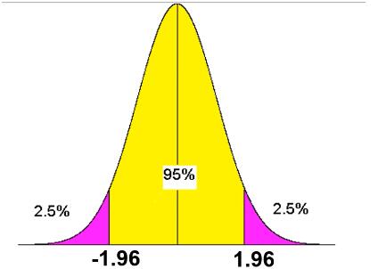
Statistic z: The area under the probability density function of the normal distribution is the probability value of the distribution function. The abscissa value of the density function corresponding to the probability value is the statistic z.

Critical value: As shown in the figure below, we define the areas of 2.5% on both the left and right sides as small probability events, that is, the purple parts are small probability events. The abscissas of the critical values of these two purple regions are: \(z = \pm 1.96\), which are called the critical values of the statistic z. When the value of the statistic z calculated from the sample is less than or greater than the critical value, the null hypothesis can be rejected.

So how to calculate the statistic of a sample? ztest in the statsmodels.stats.weightstats library can achieve this process.

The input parameters included in the ztest function are as follows:

• x1: The data values of the sample.

• value: The mean of the population in the null hypothesis.

The null hypothesis \(H_0\) of this function is that the mean corresponding to the sample x1 is value; the alternative hypothesis \(H_1\) is that the mean corresponding to the sample x1 is not value. The following output values can be obtained through the function:

• tstats: The value of the statistic

• pvalue: The p-value

If there is a sample set arr here, let’s use hypothesis testing to infer whether the mean of the population corresponding to this sample is 39.

First, let’s define a sample set with a sample size exceeding 30, because only the mean of a sample set with a size exceeding 30 can be inferred using the z-test.

arr = [23, 36, 42, 34, 39, 34, 35, 42, 53, 28, 49, 39, 46, 45, 39, 38, 45, 27,
       43, 54, 36, 34, 48, 36, 47, 44, 48, 45, 44, 33, 24, 40, 50, 32, 39, 31]
len(arr)

36

Next, let’s use ztest to calculate the statistic z corresponding to the null hypothesis:

import statsmodels.stats.weightstats as sw

# 原假设为总体的平均值是 39
z, p = sw.ztest(arr, value=39)
z

0.3859224924939799

From the results, we can see that the statistic z of the null hypothesis is 0.38, which is just greater than -1.96 and less than 1.96. Therefore, we should accept the null hypothesis.

In summary, we can conclude that the mean of the population corresponding to the sample is equal to 39.

If we change the null hypothesis to: the mean of the population corresponding to the sample is 20. Let’s recalculate the statistic t:

z, p = sw.ztest(arr, value=20)
z

15.050977207265216

From the results, it can be seen that the value of z is much greater than 1.96. Therefore, we should reject this hypothesis and accept the corresponding alternative hypothesis, that is, the mean of the population is not equal to 20.

Of course, the above z-test scheme is just one type of z-test. We can also classify z-test types into {left-tailed test, right-tailed test, and two-tailed test} according to three possibilities: {the critical value only exists on the left, the critical value only exists on the right, and the critical value exists on both sides}.

Using the statistic to determine whether to reject the null hypothesis is not the only method. We can also use the p-value to make this judgment. The p-value is the second parameter returned by the above function.

We generally believe that if the p-value is less than the significance level (0.05, that is, the probability corresponding to the critical value), it means rejecting the null hypothesis. If the p-value is greater than the significance level, the null hypothesis is accepted. You can output the above p-value to check whether the result of judging the hypothesis using the p-value is consistent with the result of judging using the statistic.

In fact, the scheme of using the p-value to judge whether the null hypothesis should be accepted is better than the scheme of judging according to the critical statistic. Because no matter which comparison distribution we choose, we can set its significance level to 0.05 (i.e., the probability of the smallest event). However, since the statistic under the distribution function corresponding to the same probability varies according to the different distribution functions. That is, the critical statistics of different comparison distributions are different, while the significance level is the same.

Therefore, everyone prefers to use the p-value to judge whether to accept the null hypothesis. Instead of calculating the statistic, then finding the critical value of the corresponding distribution function, then making a comparison, and finally drawing a conclusion.

In fact, hypothesis testing is the most important part of statistics and it also contains many knowledge points. However, since these knowledge points are not frequently used in machine learning (they are often used in data analysis), they will not be elaborated here.

90.17. Summary

This experiment first explained the three major formulas in probability theory, which are frequently used in the Naive Bayes algorithm. Then, it explained the specific differences between discrete distributions and continuous distributions, as well as the formulas and graphs of common distribution functions. Finally, it gave relevant explanations and implementations of hypothesis testing in statistics.

---

○ Sharethis article link to your social media, blog, forum, etc. More external links will increase the search engine ranking of this site.

If you find this content helpful, you can buy me a coffee

Previous

89. Python Calculus Basics

Next

91. A Concise Guide to Jupyter Notebook