
18. Support Vector Machine Implementation and Application#
18.1. Introduction#
In the previous experiments, we gave a simple introduction and experimental operations on the data processing methods for linearly distributed and non-linearly distributed data. Currently, there is another machine learning method that has shown many unique advantages in solving small sample, non-linear, and high-dimensional pattern recognition. At the same time, it can be applied not only to linearly distributed data but also to non-linearly distributed data. Compared with other basic machine learning classification algorithms such as logistic regression, KNN, naive Bayes, etc., its final performance generally outperforms these methods.
18.2. Key Points#
Linear Classification Support Vector Machine
Lagrangian Duality
-
Linear Support Vector Machine Classification Implementation
-
Nonlinear Classification Support Vector Machine
Kernel Trick and Kernel Function
18.3. Linear Classification Support Vector Machine#
In the logistic regression experiment, we tried to complete the classification for linearly separable data with a straight line. At the same time, the experiment found the optimal separation boundary by minimizing the logarithmic loss function, which is the purple straight line in the following figure.
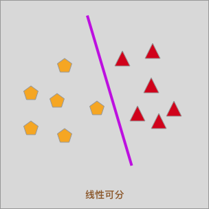
Logistic regression is a simple and efficient linear classification method. In this experiment, we will come into contact with another idea for classifying linearly separable data, and we call this method Support Vector Machine (SVM for short).
If you come across the name Support Vector Machine for the first time, it might seem a bit awkward to pronounce. At least when I first encountered Support Vector Machine, I had absolutely no idea why it had such a strange name. If you’re like I was back then, you should have a better understanding of the term Support Vector Machine after reading the following introduction.
18.4. Classification Features of Support Vector Machine#
Suppose a training dataset \(T = \{(x_1, y_1), (x_2, y_2), \cdots, (x_n, y_n)\}\) is given. Also, assume that a separating plane in the sample space has been found, and its partitioning formula can be described by the following linear equation:
When using a straight line to classify a linearly separable dataset, we already know that there may be many such straight lines:
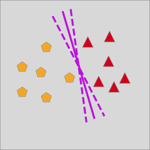
The question is, which straight line is the optimal partitioning method?
In logistic regression, we introduced the sigmoid curve and the logarithmic loss function for optimization and solution. Now, support vector machines provide a more intuitive geometric approach for solution, as shown in the following figure:
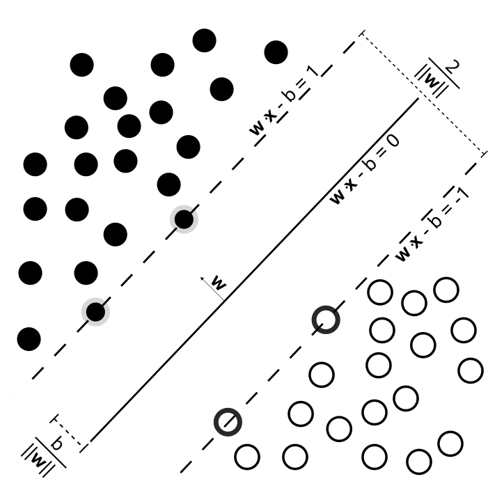
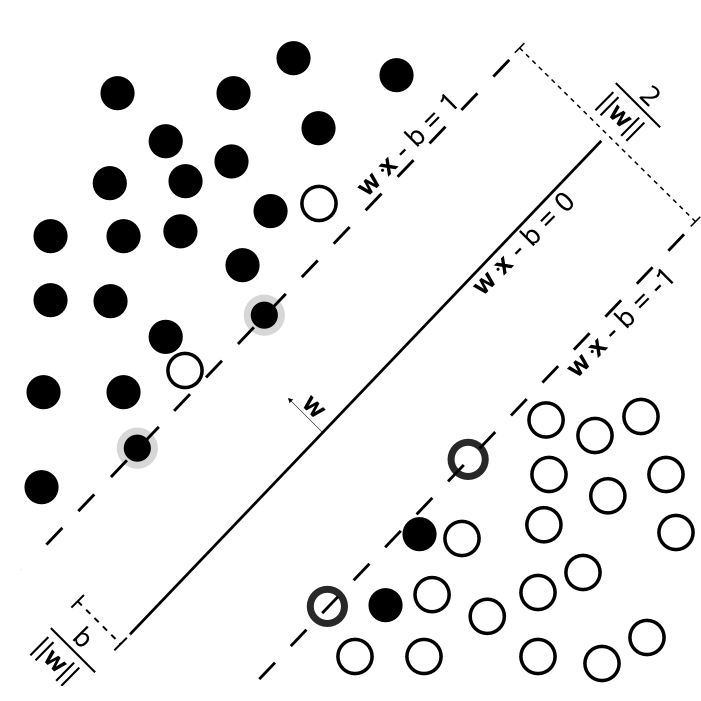
The above figure shows the process of support vector machine classification. In the figure, \(wx + b = 0\) is the separating line, and we use this line to separate the data points. At the same time, when making the separation, two parallel dotted lines are set up on both sides of the line, and the distances from these two dotted lines to the separating line are the same. This distance is often referred to as the “margin” by us. The characteristic of the support vector machine’s separation is to maximize the margin between the separating line and the dotted lines. That is, to maximize the margin between the two dotted lines.
For linearly separable positive and negative sample points, the points outside the dotted line \(wx + b = 1\) are positive sample points, and the points outside the dotted line \(wx + b = -1\) are negative sample points. Additionally, the sample points exactly on the two dotted lines are called support vectors, which is the origin of the name of the support vector machine.
18.5. Support Vector Machine Classification Demonstration#
Next, we use Python code to demonstrate the classification process of the support vector machine.
First, we introduce a new method for generating sample data.
That is, we use the
make_blobs
method provided by scikit-learn to generate clustered data.
from sklearn.datasets import make_blobs
import matplotlib.pyplot as plt

%matplotlib inline

x, y = make_blobs(n_samples=60, centers=2, random_state=30, cluster_std=0.8)  # 生成示例数据

plt.figure(figsize=(10, 8))  # 绘图
plt.scatter(x[:, 0], x[:, 1], c=y, s=40, cmap="bwr")
<matplotlib.collections.PathCollection at 0x155d430a0>

Next, we draw any 3 dividing lines in the sample data to separate the sample data.
import numpy as np

plt.figure(figsize=(10, 8))
plt.scatter(x[:, 0], x[:, 1], c=y, s=40, cmap="bwr")

# 绘制 3 条不同的分割线
x_temp = np.linspace(0, 6)
for m, b in [(1, -8), (0.5, -6.5), (-0.2, -4.25)]:
    y_temp = m * x_temp + b
    plt.plot(x_temp, y_temp, "-k")

Then, the classification margin can be manually drawn using
the
fill_between
method.
plt.figure(figsize=(10, 8))
plt.scatter(x[:, 0], x[:, 1], c=y, s=40, cmap="bwr")

# 绘制 3 条不同的分割线
x_temp = np.linspace(0, 6)
for m, b, d in [(1, -8, 0.2), (0.5, -6.5, 0.55), (-0.2, -4.25, 0.75)]:
    y_temp = m * x_temp + b
    plt.plot(x_temp, y_temp, "-k")
    plt.fill_between(x_temp, y_temp - d, y_temp + d, color="#f3e17d", alpha=0.5)

In the above figure, parameters are manually specified to present the effect of the classification margin.
As can be seen from the above drawing, the sizes of the margins corresponding to different dividing lines are inconsistent, and the goal of the support vector machine is to find the dividing line corresponding to the largest classification margin. Here, this margin refers to the geometric margin between the classification points and the hyperplane. At the same time, if you need to understand the solution principle of the support vector machine, another related concept needs to be introduced: the functional margin.
{note}
The following derivation process of the support vector machine is relatively complex. You can try to master it according to your own mathematical foundation, but it is not mandatory.
18.6. Functional Margin#
How is a sample point classified and judged in a support vector machine? When the hyperplane \(w^{T}x + b = 0\) is determined, the distance from the sample point to the hyperplane can be represented by \(|w^{T}x + b|\), and the correctness of the classification is judged by observing whether the signs of \(w^{T}x + b\) and the class \(y\) of the sample point are the same.
This process can be represented by the sign of the formula \((y - \frac{(m + n)}{2})(w^{T}x + b)\). Here, \(m\) and \(n\) are the class values of two sample points respectively, and \(y\) can be either \(m\) or \(n\). This formula can be used to judge the classification of any point. Thus, we introduce the concept of the functional margin here.
First, we define the formula for the functional margin. To simplify the formula, we define the classes \(m = 1\) and \(n = -1\) here:
Each sample point \((x_i, y_i)\) in the set \(T\) has a functional margin with respect to the hyperplane \((w, b)\). The minimum value among them is the functional margin of the hyperplane \((w, b)\) with respect to the set \(T\), which is defined as follows:
The functional margin of all points to the hyperplane is \(\geq h_{1}\). Given the minimum functional margin \(h_{1}\), can we directly use it to determine the hyperplane now? Of course not. Here, we need to mention the limitations of the functional margin.
In fact, you should also be able to see a problem with our definition of the functional margin formula here. When we change the values of \(w\) and \(b\) proportionally, \(f(x)\) will also change in proportion, but the hyperplane \((w, b)\) will not change. The mechanism of the support vector machine is to find the maximum classification margin. If the margin can be changed arbitrarily while the hyperplane does not change accordingly, then this measure is meaningless.
Therefore, only the functional margin is not enough. It would be great if there was a method to constrain the normal vector \(w\). Fortunately, the geometric margin mentioned earlier can help us solve this problem.
18.7. Geometric Margin#
We define a point \(x\), and its perpendicular projection point on the hyperplane is \(x_0\). The distance between the two points is \(h\), and \(w\) represents the normal vector of the hyperplane. As shown in the following figure:
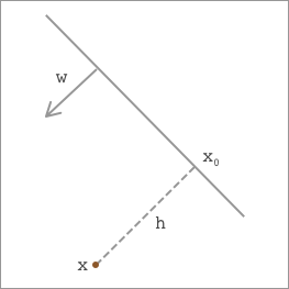
According to plane geometry knowledge, we have:
Among them, \(\frac{w}{\left \| w \right \|}\) is not difficult to understand. Dividing a vector by its norm represents the unit vector. At this time, multiplying both sides of the formula by a \(w\) gives:
In addition, as can be seen from the figure, \(x_0\) is a point on the hyperplane and satisfies \(f(x_0)=0\). Therefore, substituting it into the hyperplane gives \(w^{T}x_0 + b = 0\). Finally, substituting into the above formula to solve for the distance \(h\) yields the following result:
The above formula is easy to understand. We all know that the distance formula from a point to a line in a plane is \(D = \frac{Ax_{0}+By_{0}+C}{\sqrt{A^{2}+B^{2}}}\), which is consistent with the above when extended to higher dimensions. Here, to obtain the absolute value of the distance \(h\), we need to multiply by the class \(y\), resulting in the following:
As can be seen from the equation, there is a constraint on the normal vector \(w\) in the geometric margin. \(h_{1}\), which is the functional margin we obtained above, is just an artificially defined distance, while the geometric margin \(\left | h \right |\) is the intuitive distance from a point to the hyperplane. Its value will not change with the scaling of \(w\) and \(b\), but only with the change of the hyperplane.
From the above introduction, it can be seen that dividing the functional margin by \(\left \| w \right \|\) gives the geometric margin, and the essence of the functional margin can actually be understood as \(\left | f(x) \right |\).
18.8. Lagrangian Duality#
After having a certain understanding of the functional margin and the geometric margin, now we are faced with another problem: how to solve this optimization problem of the classification margin.
As mentioned before, due to the scaling problem of the functional margin \(h_{1}\), it is not suitable as the value to maximize the margin, so the geometric margin \(h\) is introduced to solve this problem. Therefore, here we can define the objective function for maximizing the classification margin as follows:
Since the functional margin of each point is greater than or equal to the minimum functional margin, the following constraint conditions need to be satisfied simultaneously:
We set the functional margin \(h_{1}\) to 1, and obtain the following quadratic programming problem:
In the quadratic programming problem, the part in front is the objective function, and the part after \(s.t.\) is the constraint condition.
Meanwhile, for the convenience of subsequent operations, the objective function is equivalently transformed into \(min \frac{1}{2}\left \| w \right \|^{2}\), and the following convex quadratic programming problem is obtained:
Therefore, the above formula can be expressed as: maximize the geometric margin \(\frac{1}{\left \| w \right \|}\) under the constraint conditions \(y_{i}(w^{T}x_{i}+b)-1\geq 0\: \: (i=1,2,...,n)\).
For the convenience of formula derivation, we directly “set the functional margin \(h_{1}\) to 1” to obtain the expression of the quadratic programming problem. Then, will this affect the results of subsequent operations?
First, it can be simply understood through the properties of the functional margin. As mentioned before, the functional margin can be stretched arbitrarily. Second, it can also be understood through the substitution method. Replace \(w\) with \(\frac{w}{h_{1}}\), \(b\) with \(\frac{b}{h_{1}}\), and naturally \(h_{1}\) becomes 1. Similarly, the objective function needs to be replaced.
Currently, we have obtained the expression of the convex quadratic programming problem of the support vector machine, and next we can solve it. For such a special form of structure, the usual approach is to use Lagrangian duality to transform the original problem into its dual problem, that is, to obtain the optimal solution of the original problem by solving the dual problem equivalent to the original problem. This method will make the original problem easier to solve and more naturally introduce the kernel function to solve non-linear problems subsequently.
Under the condition of satisfying the condition, Lagrangian duality incorporates the constraint conditions into the objective function by adding a Lagrange multiplier \(\lambda\) to each constraint condition, and expresses the problem through only one function. Therefore, the above convex quadratic programming problem is transformed as follows:
Now the problem is simplified, and we only need to maximize \(L\):
How does the above combined objective function equivalently solve our problem?
When a certain constraint is not satisfied, that is, when the functional margin is less than 1, as long as \(\lambda_{i}\) is defined large enough, \(L\) approaches infinity. When all constraints are satisfied, the optimal value is expressed as \(\frac{1}{2}\left \| w \right \|^{2}\), which is exactly the quantity we initially needed to minimize. Because when \(x_{i}\) is a support vector, \((y_{i}(w^{T}x_{i}+b)-1)=0\), and at this time the optimal value is \(\frac{1}{2}\left \| w \right \|^{2}\); when \(x_{i}\) is a non-support vector, the functional margin must be greater than 1, and \(\lambda_{i}\) takes non-negative values. To satisfy the maximization, \(\lambda_{i}\) must be equal to 0, and the optimal value at this time is still \(\frac{1}{2}\left \| w \right \|^{2}\).
In fact, through the above explanation, we can also find some very interesting conclusions. That is, when the constraints are satisfied, the \(\lambda\) values of non-support vectors are all equal to 0, and the whole part behind is 0; although there are infinitely many values for the \(\lambda\) of support vectors, because the functional margin is equal to 1, the whole part behind still takes a value of 0.
After a series of equivalent transformations, now we can summarize the objective function as follows:
If we directly solve the objective function at this time, it is not that easy because \(\lambda\) is a constraint of the inequality, and we still have to deal with the two parameters \(w\) and \(b\). So the usual approach is to convert it into a dual problem and exchange the positions of the max-min optimization:
Of course, the positions of the formulas cannot be exchanged randomly and certain conditions need to be met. When both the primal problem and the dual problem have optimal solutions, we can obtain:
For all optimization problems, the above formula holds. Even if the primal problem is non-convex, this property is called weak duality. Of course, there is also strong duality corresponding to it. Strong duality needs to satisfy:
In the support vector machine, after satisfying the Slater condition and the KKT condition, we directly assume that strong duality holds and solve the dual problem to obtain the solution of the primal problem. After verifying that the conditions are satisfied, we can solve for the optimal value \(d^{*}\) of the second formula.
18.9. Dual Problem Solving#
The solution of \(d^{*}\) can be carried out in two parts. However, due to the need for strong logic and a solid foundation in mathematical knowledge, this part is not required. In fact, after understanding the three contents introduced above, you should have a good grasp of the mathematical principles of the support vector machine.
On the premise of fixing \(\lambda\), take the partial derivatives with respect to \(w\) and \(b\) to minimize \(L\) with respect to \(w\) and \(b\), and set the derivatives to 0, we can get:
Now substitute the two equations into the above \(L\) to obtain the final formula:
So now our problem has become this dual form:
Currently, there is only one variable \(\lambda\) in the problem. Next, the sequential minimal optimization algorithm can be used to solve for this Lagrange multiplier.
The Sequential Minimal Optimization (SMO) algorithm was invented by John Platt of Microsoft Research in 1998 and is currently widely used in the training process of SVM. Previously available SVM training methods had to use complex methods with large computational requirements and required expensive third-party quadratic programming tools. The SMO algorithm, however, better avoids this problem.
Simply put, its idea is to optimize only two variables in one iteration while fixing the remaining variables. Thus, a large optimization problem is decomposed into several small optimization problems, and these small optimization problems are often easier to solve.
Although the sequential minimalization algorithm plays a powerful role in solving support vector machines, it also brings more complex mathematical derivations compared to the first step. Therefore, in this experiment, there will be no extensive description of it. Students with a certain mathematical foundation and those who want to delve deeper can consult relevant materials on their own or refer to the links provided in this experiment for learning.
18.10. Implementation of Linear Support Vector Machine Classification#
Above, we deduced the process of function margin, geometric margin, and solving using Lagrangian duality in support vector machines. The derivation process goes from simple to complex, so it is not necessary to master all of it, but at least one should know the meaning of function margin and geometric margin in support vector machines.
Next, we will use Python to conduct a hands-on practice on the process of support vector machines to find the maximum margin. Since the pure Python implementation of support vector machines is too complex, in this experiment, we will directly use scikit-learn to complete it.
The classes and parameters corresponding to the support vector machine classifier in scikit-learn are:
sklearn.svm.SVC(C=1.0, kernel='rbf', degree=3, gamma='auto', coef0=0.0, shrinking=True, probability=False, tol=0.001, cache_size=200, class_weight=None, verbose=False, max_iter=-1, decision_function_shape='ovr', random_state=None)
The main parameters are as follows:
-
C: The corresponding penalty parameter in the support vector machine. -
kernel: The kernel function, optional values are linear, poly, rbf, sigmoid, precomputed, which will be introduced in detail below. -
degree: The exponent of the poly polynomial kernel function. -
tol: The tolerance for convergence to stop.
As shown in the figure below, in the support vector machine,
when the training dataset is not completely linearly
separable, overfitting will occur after ensuring that each
point is correctly separated. To solve the overfitting
problem, a penalty factor
\(\xi\) is
introduced, which can be regarded as the above parameter
C, allowing a small number of points to be misclassified. In
the case where the training set is not completely linearly
separable, we should make the geometric margin as large as
possible while minimizing the number of misclassified
points.
C
is the coefficient that reconciles the two.
When we use the support vector machine to solve such problems, the maximum margin is called the maximum “soft margin”, and the soft margin means that sporadic noisy data can be misclassified. The maximum margin that can perfectly separate the data in the above text is called the “hard margin”.
Here, we still use the example data generated above to train
the support vector machine model. Since the data is linearly
separable, the
kernel
parameter can be specified as
linear.
First, train the support vector machine linear classification model:
from sklearn.svm import SVC

linear_svc = SVC(kernel="linear")
linear_svc.fit(x, y)
SVC(kernel='linear')In a Jupyter environment, please rerun this cell to show the HTML representation or trust the notebook.
On GitHub, the HTML representation is unable to render, please try loading this page with nbviewer.org.
SVC(kernel='linear')
For the trained model, we can output its corresponding
support vectors through the
support_vectors_
attribute:
linear_svc.support_vectors_
array([[ 2.57325754, -3.92687452],
       [ 2.49156506, -5.96321164],
       [ 4.62473719, -6.02504452]])
It can be seen that there are a total of 3 support vectors. If you output the coordinate values of \(x\) and \(y\), you can see the data corresponding to these 3 support vectors.
Next, we can use Matplotlib to plot the dividing line and
margin corresponding to the trained support vector machine.
To facilitate reuse later, the plotting operation is written
into the
svc_plot()
function here:
def svc_plot(model):
    # 获取到当前 Axes 子图数据,并为绘制分割线做准备
    ax = plt.gca()
    x = np.linspace(ax.get_xlim()[0], ax.get_xlim()[1], 50)
    y = np.linspace(ax.get_ylim()[0], ax.get_ylim()[1], 50)
    Y, X = np.meshgrid(y, x)
    xy = np.vstack([X.ravel(), Y.ravel()]).T
    P = model.decision_function(xy).reshape(X.shape)

    # 使用轮廓线方法绘制分割线
    ax.contour(X, Y, P, colors="green", levels=[-1, 0, 1], linestyles=["--", "-", "--"])

    # 标记出支持向量的位置
    ax.scatter(
        model.support_vectors_[:, 0], model.support_vectors_[:, 1], c="green", s=100
    )
# 绘制最大间隔支持向量图
plt.figure(figsize=(10, 8))
plt.scatter(x[:, 0], x[:, 1], c=y, s=40, cmap="bwr")
svc_plot(linear_svc)

As shown in the figure above, the solid green line represents the finally found dividing line, and the interval between the green dashed lines is the maximum margin. At the same time, the green solid dots represent the positions of the 3 support vectors.
The above data points can be linearly separable. So, what will happen if we add noise to make the data set imperfectly linearly separable?
Next, let’s handle the classification process of the support vector machine with noisy points:
# 向原数据集中加入噪声点
x = np.concatenate((x, np.array([[3, -4], [4, -3.8], [2.5, -6.3], [3.3, -5.8]])))
y = np.concatenate((y, np.array([1, 1, 0, 0])))

plt.figure(figsize=(10, 8))
plt.scatter(x[:, 0], x[:, 1], c=y, s=40, cmap="bwr")
<matplotlib.collections.PathCollection at 0x155f04a90>

It can be seen that two noise points are mixed into each of the red and blue data clusters at this time.
Train the support vector machine model at this time and draw the dividing line and the maximum margin:
linear_svc.fit(x, y)  # 训练

plt.figure(figsize=(10, 8))
plt.scatter(x[:, 0], x[:, 1], c=y, s=40, cmap="bwr")
svc_plot(linear_svc)

Due to the inclusion of noise points, the number of support vectors has changed from 3 to 11 at this time.
In the previous experiment, we mentioned the penalty coefficient \(C\). Next, we can observe the change process of the support vectors by changing the value of \(C\). At the same time, we need to introduce a module that can implement interactive operations in the Notebook. You can view the effect of the final drawing by selecting different values of \(C\).
from ipywidgets import interact
import ipywidgets as widgets


def change_c(c):
    linear_svc.C = c
    linear_svc.fit(x, y)
    plt.figure(figsize=(10, 8))
    plt.scatter(x[:, 0], x[:, 1], c=y, s=40, cmap="bwr")
    svc_plot(linear_svc)


interact(change_c, c=[1, 10000, 1000000])
<function __main__.change_c(c)>
18.11. Nonlinear Classification Support Vector Machine#
In the above content, we assumed that the samples are linearly separable or not strictly linearly separable, and then implemented sample classification by establishing support vector machines in these two cases. However, linearly separable samples are often just an ideal situation, and most of the original samples in reality are linearly inseparable. In this case, can we still use the support vector machine?
Do you still remember the kernel function mentioned for handling dual problems before? In fact, for linearly inseparable data sets, we can also use support vector machines to complete classification. However, here we need to add a technique to convert linearly inseparable data into linearly separable data before completing the classification.
We call this data transformation technique the “kernel trick”, and the function that implements the data transformation is called the “kernel function”.
{note}
The kernel trick is a mathematical method. This experiment only explains its application scenario in support vector machines.
18.12. Kernel Trick and Kernel Function#
According to the above introduction, we mentioned an idea, which is the kernel trick, that is, first convert linearly inseparable data into linearly separable data, and then use support vector machines to complete the classification. So, how exactly is it operated?
The key to the kernel trick lies in space mapping, that is, mapping low-dimensional data into a high-dimensional space so that the data set can be linearly separable in the high-dimensional space.
The above sentence is not easy to understand. Let’s introduce it through an analogy:
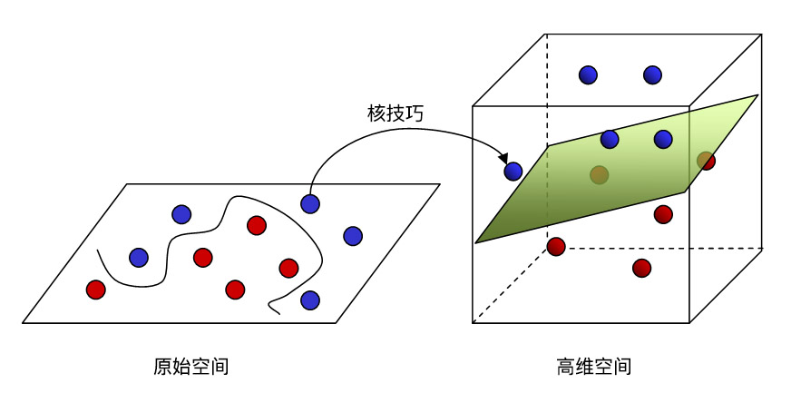
As shown in the figure above, assume that we have two types of data points represented by blue and red in a two-dimensional space. Obviously, it is impossible to separate these two types of data with a straight line. At this time, if we use the kernel trick to map it into a three-dimensional space, it becomes a state that can be linearly separable by a plane.
For the “mapping” process, we can also understand it in this way: The red and blue balls distributed on the two-dimensional desktop cannot be linearly separated. At this time, slap the palm on the desktop (it hurts so much), and the balls jump into the three-dimensional space under the action of the force. This is also an intuitive mapping process.
At the same time, the process of “mapping” is also the process of transformation through the kernel function. Here, it needs to be supplemented that there are many methods to transform data points from a low-dimensional space to a high-dimensional space, but they often involve huge computational amounts. Mathematicians have discovered several special functions from them. Such functions can greatly reduce the computational complexity and are thus named “kernel functions”. That is to say, the kernel trick is a special “mapping” trick, and the kernel function is the implementation method of the kernel trick.
Next, let’s get to know several common kernel functions:
Linear kernel function:
Polynomial kernel function:
Gaussian Radial Basis Function (RBF) kernel:
Sigmoid kernel function:
These 4 kernel functions respectively correspond to the 4 different values of ‘linear’, ‘poly’, ‘rbf’,‘sigmoid’ for the ‘kernel’ parameter in the SVC method of scikit - learn introduced above.
In addition, kernel functions can also be obtained through function combination. For example:
If \(k_1\) and \(k_2\) are kernel functions, then for any positive numbers \(\lambda_1,\lambda_2\), their linear combination:
18.13. Introduction to the Margin Representation and Solution of Kernel Functions#
By directly introducing the kernel function \(k(x_i,x_j)\), without explicitly defining the high-dimensional feature space and the mapping function, we can use the method for solving linear classification problems to solve the support vector machine for nonlinear classification problems. After introducing the kernel function, the dual problem becomes:
As can be seen from the above formula, after introducing the penalty coefficient, it has the same form as the original objective function. The only difference lies in the range of \(\lambda_{i}\).
Similarly, after obtaining the optimal solution \(\lambda^{*}=\left(\lambda_{1}^{*}, \lambda_{2}^{*}, \ldots, \lambda_{N}^{*}\right)\) through the solution of the previous dual problem, based on this, we can obtain the optimal solutions \(w^{*}\) and \(b^{*}\), and thus obtain the separating hyperplane:
Using the sign function, the classification decision function between positive and negative classes is obtained as:
18.14. Nonlinear Support Vector Machine Classification Implementation#
Similarly, we use the SVC class provided in scikit-learn to build a nonlinear support vector machine model and draw the decision boundary.
First, the experiment needs to generate a set of sample
data. Above, we used
make_blobs
to generate a set of linearly separable data. Here, we use
make_circles
to generate a set of linearly inseparable data.
from sklearn.datasets import make_circles

x2, y2 = make_circles(150, factor=0.5, noise=0.1, random_state=30)  # 生成示例数据

plt.figure(figsize=(8, 8))  # 绘图
plt.scatter(x2[:, 0], x2[:, 1], c=y2, s=40, cmap="bwr")
<matplotlib.collections.PathCollection at 0x156bd56f0>

The above figure is obviously a set of linearly inseparable data. When we train the support vector machine model, we need to introduce the kernel trick. For example, we use the following formula to make a simple non-linear mapping here:
def kernel_function(xi, xj):
    poly = xi**2 + xj**2
    return poly
from mpl_toolkits import mplot3d
from ipywidgets import interact, fixed

r = kernel_function(x2[:, 0], x2[:, 1])
plt.figure(figsize=(10, 8))
ax = plt.subplot(projection="3d")
ax.scatter3D(x2[:, 0], x2[:, 1], r, c=y2, s=40, cmap="bwr")
ax.set_xlabel("x")
ax.set_ylabel("y")
ax.set_zlabel("r")
Text(0.5, 0, 'r')

The above shows the effect of mapping points in a two-dimensional space to a high-dimensional space. Next, we use the RBF (Radial Basis Function) kernel function provided by the SVC method in sklearn to complete the experiment.
rbf_svc = SVC(kernel="rbf", gamma="auto")
rbf_svc.fit(x2, y2)
SVC(gamma='auto')In a Jupyter environment, please rerun this cell to show the HTML representation or trust the notebook.
On GitHub, the HTML representation is unable to render, please try loading this page with nbviewer.org.
SVC(gamma='auto')
plt.figure(figsize=(8, 8))
plt.scatter(x2[:, 0], x2[:, 1], c=y2, s=40, cmap="bwr")

svc_plot(rbf_svc)

Similarly, we can challenge different penalty coefficients \(C\) to see the changes in the decision boundary and support vectors:
def change_c(c):
    rbf_svc.C = c
    rbf_svc.fit(x2, y2)
    plt.figure(figsize=(8, 8))
    plt.scatter(x2[:, 0], x2[:, 1], c=y2, s=40, cmap="bwr")
    svc_plot(rbf_svc)


interact(change_c, c=[1, 100, 10000])
<function __main__.change_c(c)>
18.15. Multi-class Support Vector Machine#
Support vector machines were originally designed for binary classification problems. When we face multi-class classification problems, we can actually use support vector machines to solve them as well. The solution is to construct a multi-class classifier by combining multiple binary classifiers. According to the construction method, it can be divided into two methods:
-
One-vs-rest method: That is, during training, the samples of a certain category are classified into one category in turn, and the remaining samples are classified into another category. In this way, \(k\) support vector machines are constructed for the samples of \(k\) categories.
-
One-vs-one method: That is, a support vector machine is constructed between any two categories of samples. Therefore, \(k(k - 1) \div 2\) support vector machines need to be designed for the samples of \(k\) categories.
In scikit-learn, implementing a multi-class support vector
machine is determined by setting the parameter
decision_function_shape, where:
-
decision_function_shape='ovo': Represents the one-vs-one method. -
decision_function_shape='ovr': Represents the one-vs-rest method.
Since only the parameters need to be modified here, there is no need to elaborate further.
Finally, let’s summarize the advantages and disadvantages of SVM. First of all, SVM is a very good method, especially for non-linear classification problems. Moreover, the biggest disadvantage lies in the computational efficiency. As the dataset increases, the computational time increases steeply. Therefore, generally we will apply SVM to small datasets, while large datasets are basically not considered.
18.16. Summary#
In this experiment, we learned what a support vector machine is and explored function margin, geometric margin, Lagrangian duality, as well as the characteristics and usage methods of kernel functions. As is well known in the field of machine learning, the support vector machine is an algorithm that is easy to understand but difficult to delve into deeply. Although the experiment tried to present some mathematical principles from simple to complex, this experiment still recommends only mastering the usage method of the SVC class in scikit-learn. Of course, for students with a better mathematical foundation, they can try to derive the implementation process of SVM by themselves.
Related Links