
70. Principles of Recurrent Neural Networks#
70.1. Introduction#
In this section of the experiment, we will start learning about Recurrent Neural Networks (RNNs). Recurrent neural networks have achieved great success and are widely used in fields such as natural language processing and speech recognition. They have significant advantages in processing sequence models, and have gradually enabled deep learning to be successfully applied in more fields.
70.2. Key Points#
Introduction to Sequence Models
Simple Recurrent Neural Networks
LSTM (Long Short-Term Memory) Model
GRU (Gated Recurrent Unit)
70.3. Introduction to Natural Language Processing#
In natural language processing, “natural language” refers to the language that occurs naturally, that is, the language used in daily communication by people. Language is the essential characteristic that differentiates humans from other animals. Among all living beings, only humans have the ability to process and understand language. The logical thinking of humans takes the form of language, and the vast majority of human knowledge is also recorded and passed down in the form of language and writing.
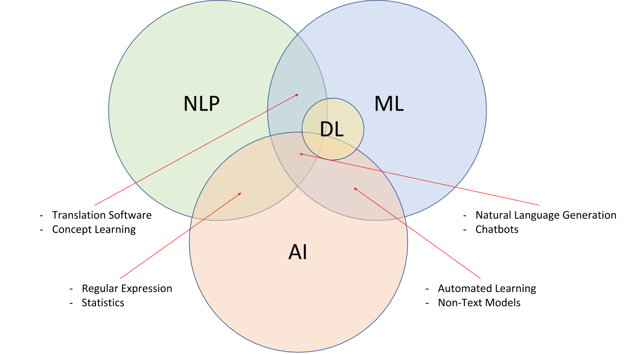
Natural language processing is not only an application field of computational linguistics, but also an important research direction in the fields of computer science and artificial intelligence. Natural language processing mainly studies various theories and methods for effective communication between humans and computers using natural language. Therefore, natural language processing is actually a discipline integrating linguistics, computer science, and mathematics. NLP expert Michael Frederikse believes that natural language processing has the following intersection relationships with machine learning, deep learning, and artificial intelligence.
Although natural language processing is related to linguistics, it is different from the pure study of natural language in linguistics. Linguistics takes natural language as the research object and studies the nature, function, structure, application, historical development of language, and other issues related to language. Natural language processing lies in the study of computer systems that can effectively achieve natural language communication between humans and machines.
After years of development and progress, from the perspective of natural language, natural language processing can be divided into two parts: natural language understanding and natural language generation.
Among them, natural language understanding is a comprehensive systematic project that involves many subdivided disciplines. For example, phonology that systematically studies the pronunciation in language, morphology that studies word formation and the relationships between words, etc. Generally speaking, natural language understanding can be further divided into three aspects, namely: lexical analysis, syntactic analysis, and semantic analysis.
The generation of natural language is to automatically generate text in a reading manner from structured data (which can be popularly understood as the data after natural language understanding and analysis). There are mainly three stages:
-
Text planning: Complete the basic content planning in structured data.
-
Sentence planning: Combine sentences from structured data to express the information flow.
-
Realization: Generate grammatically correct sentences to express the text.
Currently, natural language processing has a very rich range of applications. Generally speaking, the main classifications are as follows:
-
Information retrieval: Index large-scale documents.
-
Speech recognition: Convert the acoustic signals of natural languages including spoken language into expected signals.
-
Machine translation: Translate one language into another.
-
Intelligent question answering: Automatically answer questions.
-
Dialogue system: Through multi-turn conversations, chat with users, answer questions, and complete certain tasks.
-
Text classification: Automatically classify texts.
-
Sentiment analysis: Judge the sentiment tendency of a certain text.
-
Text generation: Automatically generate texts according to requirements.
-
Automatic summarization: Summarize the abstracts of texts.
However, before truly getting into the application level of natural language, we need to first learn its most commonly used type of deep neural network: the Recurrent Neural Network.
70.4. Introduction to Sequence Models#
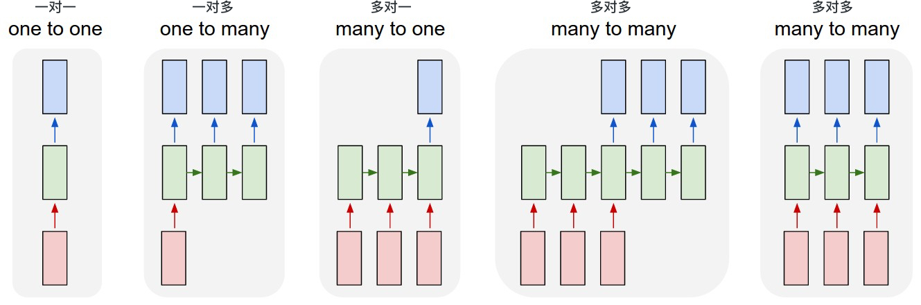
In machine learning tasks, many tasks can actually be regarded as sequence models. A sequence means that the elements in this model are no longer independent but have a certain correlation. Generally, based on the input and output, we divide the commonly used models into the following categories:
-
One-to-One Model: Our previous models, such as fully connected neural networks, have a one-to-one structure. We give it an input and it can get an output, and different inputs are regarded as independent relationships and are learned or recognized separately. Now, what we are going to focus on are the last four figures, that is, the sequential models.
-
One-to-Many Model: Based on an output of the model, it can be used to predict a sequence. For example, for an image, output a string of captions to describe it.
-
Many-to-One Model: Based on a sequential input, predict a single value. For example, based on a user’s comment in a restaurant, judge the user’s evaluation of this restaurant. Then, the input is a passage as a sequential input, and the output is a number between 0 and 5 as a score.
-
Many-to-Many with Delay: Based on the sequential input of the model, we output a sequence with a delay according to the existing input. Common tasks include learning tasks for translation, such as translating English into Chinese. The model needs to wait until the English input reaches a certain level before it can be translated into Chinese, so both the input and output are a sequence.
-
Many-to-Many without Delay: Based on the sequential input of the model, output a sequence synchronously according to the input. A common example is making weather forecasts, where it is necessary to make a prediction of the probability of rain in real time based on measured temperature, humidity, etc. However, each prediction actually also needs to consider some previous sequential inputs and is not determined only by the input at this moment.
It can be seen that the typical characteristic of sequence models is that the input and output are not independent, and the output is often related to the input of the previous step or even the previous several steps. Considering the existence of such models and in order to better fit such a process, the Recurrent Neural Network (RNN) came into being.
70.5. Simple Recurrent Neural Network#
In traditional neural networks, each layer from the input layer to the output layer is fully connected directly, but the neurons within a layer have no connections with each other. It is indeed difficult to apply this network structure to many scenarios, such as text processing and speech translation.
The solution of the Recurrent Neural Network (RNN) is to make the hidden layer consider not only the output of the previous layer but also the output of this hidden layer at the previous moment. In theory, the RNN can include the states at any number of previous moments. In practice, to reduce the complexity of the model, we generally only process the outputs of the previous few states.
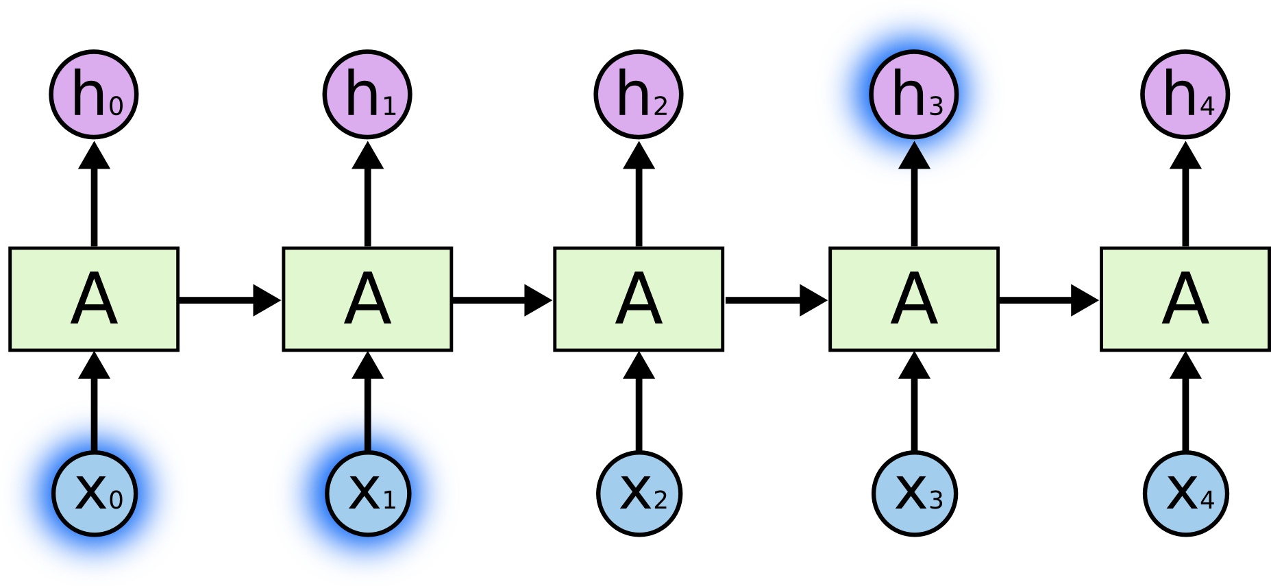
Compared with traditional feedforward neural networks, the Recurrent Neural Network (RNN) connects the same layer at different time series back and forth. In terms of weights, another weight is introduced to determine how the output of the previous moment is used as input and affects the output of the next moment. Thus, there is such a simple basic structure:
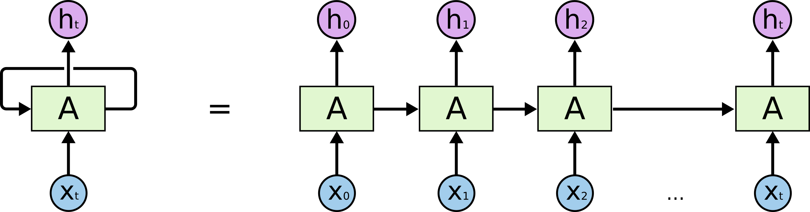
The left side represents a recurrent graph, and the right side shows the idea when building the network specifically. The two are completely equivalent. For neuron \(A\), \(X_t\) is the input and \(h_t\) is the output of the hidden layer. Among them, \(h_t\) is not only related to \(X_t\) but also affected by \(h_{t - 1}\).
At this time, you need to understand the huge difference between the input of the Recurrent Neural Network (RNN) and that of the feedforward neural network. The inputs \(x_0 \cdots x_t\) of the feedforward neural network are passed in all at once, while in the RNN, after \(x_0\) is passed in and \(h_0\) is obtained, the input of \(x_1\) is then carried out.
The following is a more complete structure diagram of the Recurrent Neural Network (RNN), from which you can clearly see how the output of each time step is calculated.
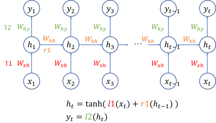
An activation function is added to the above formula. For example, if we want to obtain \(h_2\), it can be simply written as:
70.6. Long Short-Term Memory (LSTM) Model#
In the following experimental content, we referred to the illustrations and some content in Understanding LSTM Networks written by Christopher Olah.
Simple recurrent neural networks (RNNs) are generally only related to a certain number of previous sequences. If the number of steps exceeds ten, problems such as vanishing gradients or exploding gradients are likely to occur. Among them, vanishing gradients occur because, in the process of chain differentiation, due to the relatively deep depth of the related sequences, the gradients disappear exponentially.
In addition, simple recurrent neural networks cannot solve the problem of long-term dependencies. For example, when we predict “I live in ___ Shijingshan District”, the RNN may easily get the result of “Beijing”. This is because the interval between the content to be predicted and the relevant information is very small, and the recurrent neural network can use past information to obtain the prediction result.
However, if the interval between the content to be predicted and the relevant information is very long. For example, “I am a native Beijinger,… [a long paragraph is omitted here]…, my mother tongue is ____”. At this time, it is very difficult for the recurrent neural network to make an accurate prediction. Because the information dependence distance is too long, it is very difficult for the RNN to associate them.

To effectively solve this problem, the recurrent neural network can also enhance the function of the hidden layer by changing the module. Among them, LSTM and GRU are the most classic.
The full name of LSTM is Long Short-Term Memory Model, which is a very popular meta-structure of recurrent neural networks at present. It is not essentially different from the general RNN structure, except that different functions are used to calculate the state of the hidden layer.
The following figure is the structure of our previous simple RNN:
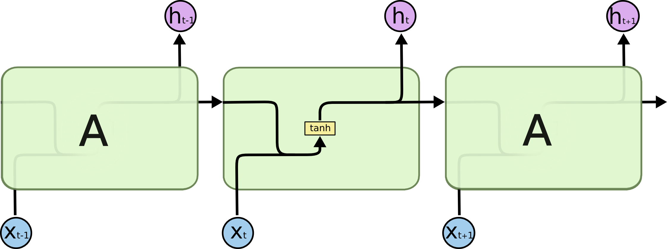
Now, we introduce the structure of LSTM. With this structure, LSTM can well solve the long-term dependence problem because it itself has the ability to remember information for a long time.
Next, let’s analyze the module connections of LSTM step by step.
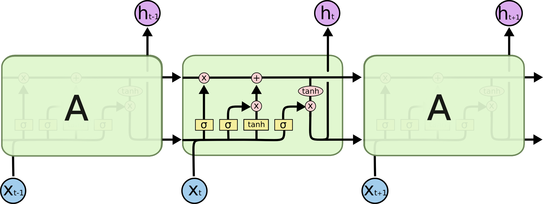
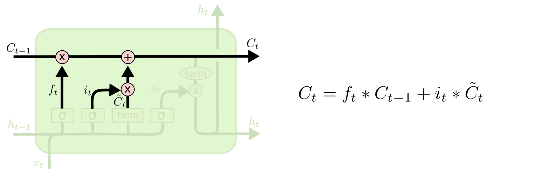
Like a connecting line, the cell state \(C\) connects LSTM modules at different time steps in time series. It may be the most essential part of LSTM. Among them, the multiplication operation controls how much of the cell state from the previous time step can enter the next time step, and the addition operation determines how the cell state is updated at this time step.
The horizontal connecting line above cannot add or delete information. LSTM achieves this through a structure called “gate”. Briefly speaking, the gate structure controls the flow of information, mainly through a sigmoid module and element-wise multiplication operations. As we all know, the sigmoid outputs a value between 0 and 1. Through element-wise multiplication, 0 can prevent any information from passing through, while 1 allows all information to pass through. There are three such gate structures in LSTM to protect and control information. They are: forget gate, input gate, and output gate.
First, let’s look at the structure of the “forget gate”. Its main function is to determine which information can continue to pass through this unit.
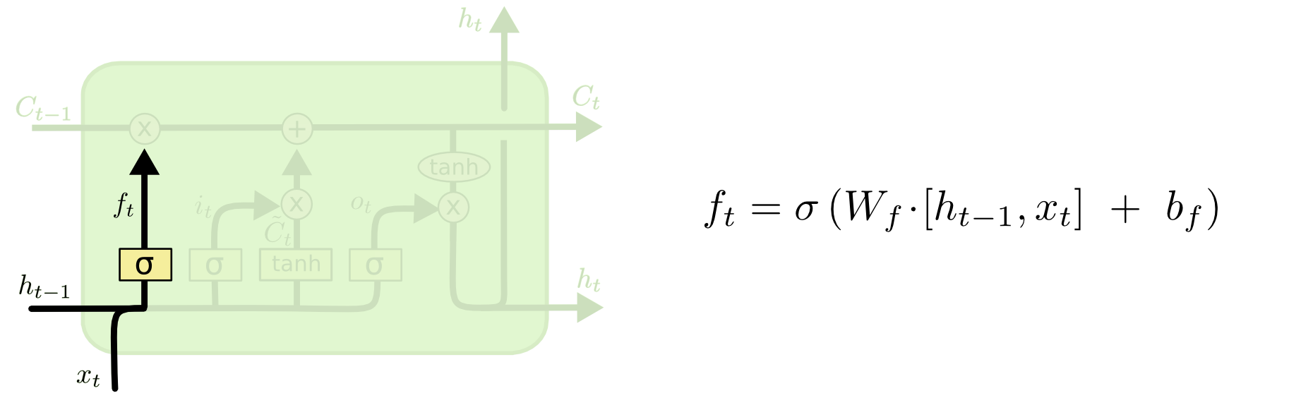
In the figure above, \(C\) represents the cell state, and the subscript \(t\) represents its values at different time steps. At the leftmost part, taking the output \(h_{t - 1}\) from the previous time step and the input \(x_{t}\) of this layer at this time step as inputs, after being activated through the sigmoid module and the corresponding weight updates therein, it outputs a value \(f_{t}\) within \([0, 1]\), which determines how much of the cell state \(C_{t - 1}\) from the previous time step can enter this time step.
Let’s turn our attention to the middle part. This part determines how much new information will be added to the cell state through the LSTM module at this time step. It consists of two parts. First, \(i_{t}\) activated by the sigmoid determines one part, and then it is multiplied by \(\tilde{C}_{t}\) activated by the tanh:
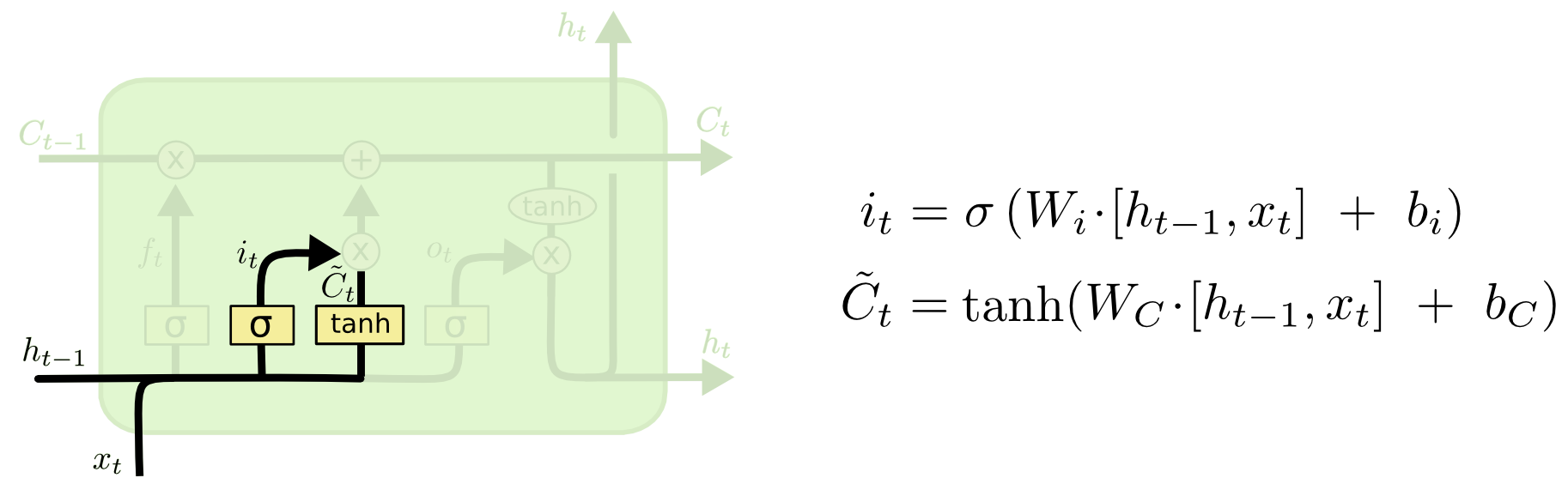
After that, by combining the forget gate result and the input gate result into the cell state, the update of the cell state can be completed. This thus constitutes the complete “input gate” structure.
After completing the update of the cell state, let’s take a look at the “output gate” structure of the LSTM. The tanh helps us push \(C_{t}\) into the range of \([-1, 1]\). By multiplying the sigmoid activation of the two inputs \(h_{t - 1}\) and \(x_{t}\), we get the final output:
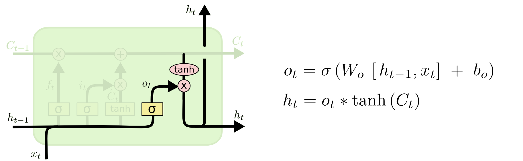
Here, let’s take a more vivid example to recap the functions of different gate structures in the LSTM. For example, when training a language model, the cell state of the LSTM should contain the gender information of the current subject so that it can correctly predict and use personal pronouns. However, when a new subject starts to be used in the sentence, the role of the forget gate is to forget the gender information of the previous subject to avoid affecting the following text. Next, the input gate needs to pass the new subject gender information into the cell.
Finally, the role of the output gate is to filter the final output. Suppose the model has just encountered a pronoun, and then it may need to output a verb, which is related to the information of the pronoun. For example, whether this verb should be in the singular or plural form requires adding all the information related to the pronoun just learned to the cell state in order to obtain the correct output.
Now, let’s summarize the parameters we need to learn in the LSTM:
Final memory cell:
Final output:
Therefore, \(W_{f}\), \(U_{f}\), \(b_{f}\); \(W_{i}\), \(U_{i}\), \(b_{i}\); \(W_{c}\), \(U_{c}\), \(b_{c}\); \(W_{o}\), \(U_{o}\), \(b_{o}\) are all variables to be learned. Similarly, their values are updated through the backpropagation method.
70.7. GRU (Gated Recurrent Unit)#
GRU stands for Gated Recurrent Unit. As mentioned before, in order to overcome the problem that RNNs cannot handle long-distance dependencies well, LSTM was proposed, and GRU is a variant of LSTM. Of course, there are many other variants of LSTM. GRU maintains the effectiveness of LSTM while making the structure simpler, so it is also very popular. Let’s take a look at the core modules of GRU.
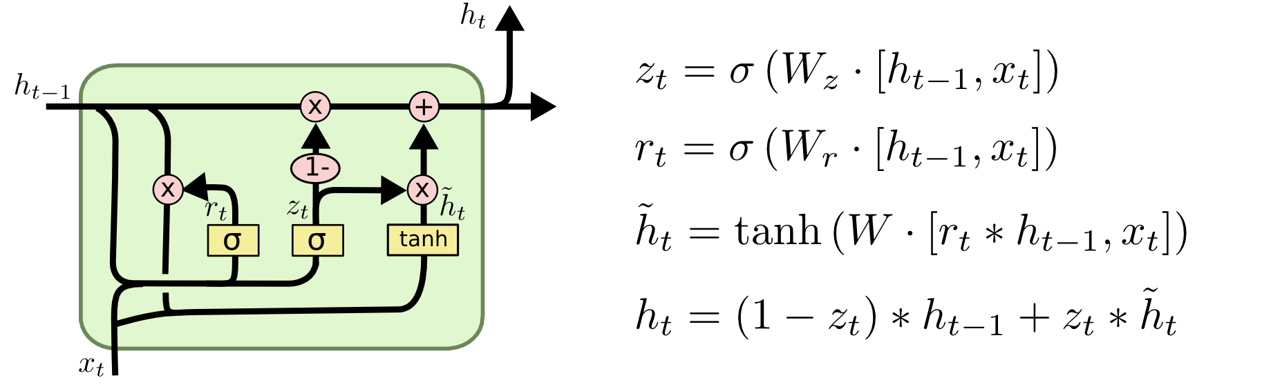
When introducing LSTM before, it was mentioned that LSTM implemented three gate calculations, namely: the forget gate, the input gate, and the output gate. As a variant of LSTM, GRU has two gates to achieve the same operations: the update gate and the reset gate, that is, \(z_{t}\) and \(r_{t}\) in the above figure. We describe the operation process of GRU according to the above figure:
The first two equations \(r_{t}\) and \(z_{t}\) calculate how much information in the GRU module needs to be forgotten and updated respectively. Then, \(\tilde{h_{t}}\) determines the current memory content. If \(r_{t}\) is 0, then \(\tilde{h_{t}}\) only retains the current information. Finally, \(z_{t}\) controls how much information needs to be forgotten from the previous moment \(h_{t - 1}\) and how much information from the current memory \(\tilde{h_{t}}\) should be added, and finally the output \(h_{t}\) at this moment is obtained.
It can be seen that a significant difference between GRU and LSTM is that GRU does not have an output control gate.
There are also many variants of LSTM. For example, the popular LSTM variant introduced by Gers, et al. (2000) adds “peephole connections”. This means that we can let the gates observe the Cell state. Another example is the Depth Gate RNN proposed by Yao, et al. (2015), and the Clockwork RNN proposed by Koutnik, et al. (2014), etc. When it comes to GRU and LSTM, GRU has fewer parameters, so it is slightly faster to train or requires less data to generalize. On the other hand, if you have enough data, the powerful expressive ability of LSTM may produce better results.
70.8. Bidirectional RNN#
In classical recurrent neural networks, the transmission of the state is unidirectional from front to back. However, in some problems, the output at the current moment is related not only to the previous state but also to the subsequent state. For example, in our usual Chinese-English translation, we can make our translation more accurate based on the context before and after. In this case, bidirectional recurrent neural networks (Bidirectional Recurrent Neural Networks) are needed to solve such problems.
The original bidirectional RNN is composed of two relatively simple RNNs stacked on top of each other. The output is jointly determined by the states of these two RNNs.
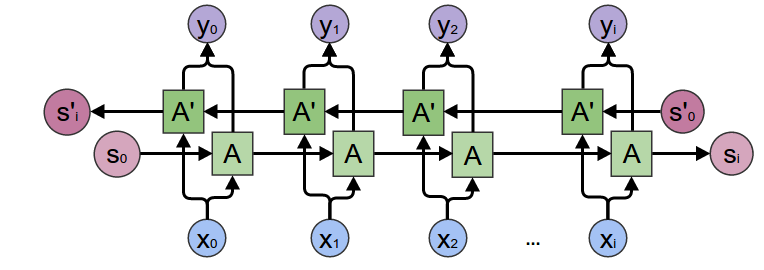
As can be seen from the above figure, the main structure of the bidirectional RNN is the combination of two unidirectional RNNs. At each time step \(t\), the input is provided to these two RNNs with opposite directions simultaneously, and the output is jointly determined by these two unidirectional RNNs. The bidirectional RNN can better simulate the bidirectional time series model, and its applications are also continuously extending and developing. For example, combining the bidirectional idea with LSTM and GRU to form bidirectional LSTM or bidirectional GRU, etc.
70.9. Deep RNN#
Deep RNNs build more complex models by stacking multiple RNN networks, as shown in the following figure.

Deep RNNs can use the ordinary RNN structure, or GRU or LSTM. In addition to the unidirectional NN, bidirectional RNNs can also be used, and their structures can be changed according to different tasks, such as the one-to-many, many-to-one, and many-to-many learning tasks we mentioned in the sequence model.
For ordinary neural networks, the number of layers can be very large, such as more than 100 layers. For deep RNNs, having three layers as shown in the above figure is already very deep because each layer of the RNN also has depth in the time dimension. Even if the number of RNN layers is not large, the overall scale of the network will be extremely huge. For deep RNNs, there is another approach. After stacking several layers of RNNs like in the above figure, the output of the RNN at each time step is input into separate ordinary deep networks, and these ordinary deep networks give the final prediction values at each time step. These ordinary deep networks are no longer connected in the time dimension like the RNN.
In conclusion, the structure of RNNs is very flexible, and both academia and industry are continuously conducting in-depth research on RNNs. It is believed that more new structures will further enhance our deep learning’s fitting and generalization capabilities.
70.10. Summary#
In this experiment, we learned about the relevant knowledge of recurrent neural networks. Similar to convolutional neural networks, recurrent neural networks currently also have relatively clear application scenarios and development momentum, and are one of the indispensable means in natural language processing, speech recognition, etc. The basic structure of recurrent neural networks is simple, but there are rich variants. Hojjat Salehinejad et al. summarized the important development nodes of recurrent neural networks in the paper Recent Advances in Recurrent Neural Networks. You can read it if you are interested.
Related Links