
97. SciPy Scientific Computing Basics#
97.1. Introduction#
SciPy is an open-source library for mathematics, science, and engineering, integrating modules such as statistics, optimization, linear algebra, Fourier transforms, signal and image processing, and ODE solvers. It is one of the important tools for scientific computing using Python. This course will introduce you to the basic usage of SciPy.
97.2. Key Points#
Constants module
Linear algebra
Interpolation functions
Image processing
Optimization methods
Signal processing
Statistical functions
Sparse matrices

SciPy generally represents an open-source software ecosystem for mathematical, scientific, and engineering development using Python, which includes a series of core libraries and tools such as NumPy, Pandas, Matplotlib, SymPy, IPython, etc. These tools also belong to the sponsored projects of NumFOCUS.
Of course, the SciPy mentioned in this chapter specifically refers to the SciPy core library, which is built on top of NumPy and inherits NumPy’s efficient computing capabilities for multi-dimensional data. Therefore, before learning the content of this section, it is recommended that you first study the NumPy Basic Course on Numerical Computing.
First, we import SciPy and check the version number:
import scipy

scipy.__version__
'1.13.1'
In a sense, SciPy can be regarded as an extension and supplement to NumPy. If you read the official SciPy documentation, you will also find that it mentions a lot of NumPy usage. Next, we will try to understand and master the unique content in the SciPy library and learn the commonly used modules and classes.
97.3. Constants Module#
For the convenience of scientific computing, SciPy provides
a module called
scipy.constants, which contains common physical and mathematical constants
and units. You can view these constants and units through
the link given above. Here we give a few examples.
For example, the mathematical constants of pi and the golden ratio.
from scipy import constants

constants.pi
3.141592653589793
constants.golden
1.618033988749895
Constants such as the speed of light in a vacuum and Planck’s constant, which are often used in physics.
constants.c, constants.speed_of_light # 两种写法
(299792458.0, 299792458.0)
constants.h, constants.Planck
(6.62607015e-34, 6.62607015e-34)
Regarding these constants, you don’t need to memorize each one. In fact, their names are logical and regular, mostly abbreviations of common English letters. When actually using them, just refer to the official documentation.
97.4. Linear Algebra#
Linear algebra should be one of the most frequently involved
computational methods in scientific computing. SciPy
provides detailed and comprehensive linear algebra
computational functions. These functions are basically
placed under the module
scipy.linalg. Among them, they are roughly divided into several
categories: basic solution methods, eigenvalue problems,
matrix decompositions, matrix functions, matrix equation
solving, special matrix construction, etc. Next, we will try
to use the relevant linear algebra solution functions in
SciPy.
For example, to find the inverse of a given matrix, we can
use the
scipy.linalg.inv
function. What is generally passed into the function is of
the type of the array
np.array
or matrix
np.matrix
given by NumPy.
import numpy as np
from scipy import linalg

linalg.inv(np.matrix([[1, 2], [3, 4]]))
array([[-2. ,  1. ],
       [ 1.5, -0.5]])
Singular value decomposition should be a pain point for
everyone in the process of learning linear algebra. Using
the
scipy.linalg.svd
function provided by SciPy can very conveniently complete
this process. For example, we perform singular value
decomposition on a
\(5 \times 4\)
random matrix.
U, s, Vh = linalg.svd(np.random.randn(5, 4))
U, s, Vh
(array([[-0.75119934,  0.39250178, -0.07910727,  0.47990549, -0.21230796],
        [-0.14271361, -0.60602855, -0.76526919,  0.1603031 ,  0.03206556],
        [ 0.42156309,  0.46901068, -0.48956675, -0.06906547, -0.59822061],
        [-0.41860256,  0.2416375 , -0.27300769, -0.8046263 ,  0.21077602],
        [ 0.24977758,  0.44756233, -0.30642504,  0.30298534,  0.7426996 ]]),
 array([3.35911649, 2.61360688, 1.30618213, 0.29283192]),
 array([[-0.20372706, -0.39790835,  0.04096205,  0.89358063],
        [ 0.3559683 ,  0.82078498, -0.00236764,  0.4467583 ],
        [ 0.77481996, -0.33587023,  0.53557332,  0.00253815],
        [ 0.48107784, -0.23488751, -0.84349139,  0.04375207]]))
Finally, the unitary matrices
U
and
Vh, and the singular values
s
are returned.
In addition,
scipy.linalg
also includes functions such as the least squares solution
function
scipy.linalg.lstsq. Now try to use it to complete a least squares solution
process.
First, we give the \(x\) and \(y\) values of the samples. Then assume that they conform to the distribution of \(y = ax^2 + b\).
x = np.array([1, 2.5, 3.5, 4, 5, 7, 8.5])
y = np.array([0.3, 1.1, 1.5, 2.0, 3.2, 6.6, 8.6])
Next, we calculate \(x^2\) and add the intercept term coefficient 1.
M = x[:, np.newaxis]**[0, 2]
M
array([[ 1.  ,  1.  ],
       [ 1.  ,  6.25],
       [ 1.  , 12.25],
       [ 1.  , 16.  ],
       [ 1.  , 25.  ],
       [ 1.  , 49.  ],
       [ 1.  , 72.25]])
Then use
linalg.lstsq
to perform the least squares calculation, and the first set
of parameters returned is the fitting coefficient.
p = linalg.lstsq(M, y)[0]
p
array([0.20925829, 0.12013861])
We can plot a graph to check whether the parameters obtained by the least squares method are reasonable, and draw the sample and fitting curve graphs.
from matplotlib import pyplot as plt
%matplotlib inline

plt.scatter(x, y)
xx = np.linspace(0, 10, 100)
yy = p[0] + p[1]*xx**2
plt.plot(xx, yy)
[<matplotlib.lines.Line2D at 0x1135ae490>]

The module
scipy.linalg
(https://docs.scipy.org/doc/scipy/reference/linalg.html) contains many methods related to linear algebra
operations. I hope everyone can learn about them by reading
the official documentation.
97.5. Interpolation Function#
Interpolation is a process or method in the field of
numerical analysis to deduce new data points within a range
through known and discrete data points. The module
scipy.interpolate
(https://docs.scipy.org/doc/scipy/reference/interpolate.html) provided by SciPy contains a large number of mathematical
interpolation methods, covering a very comprehensive range.
Next, we introduce the process of performing linear interpolation using SciPy, which is also the simplest one among the interpolation methods. First, we give a set of values for \(x\) and \(y\).
x = np.array([0, 1, 2, 3, 4, 5, 6, 7, 8, 9])
y = np.array([0, 1, 4, 9, 16, 25, 36, 49, 64, 81])

plt.scatter(x, y)
<matplotlib.collections.PathCollection at 0x113778510>

Next, we want to insert another value between the two points above. How can we best reflect the distribution trend of the data? At this time, the method of linear interpolation can be used.
from scipy import interpolate

xx = np.array([0.5, 1.5, 2.5, 3.5, 4.5, 5.5, 6.5, 7.5, 8.5])  # 两点之间的点的 x 坐标
f = interpolate.interp1d(x, y)  # 使用原样本点建立插值函数
yy = f(xx)  # 映射到新样本点

plt.scatter(x, y)
plt.scatter(xx, yy, marker='*')
<matplotlib.collections.PathCollection at 0x1137fb350>

It can be seen that the asterisk point is the point for our interpolation, while the dot points are the original sample points, and the interpolated point can accurately conform to the trend of the known discrete data points.
There are a very rich variety of mathematical interpolation methods. For details, please read the various methods listed in the official SciPy documentation. In fact, if you have studied The Basics of Pandas Data Processing, then you should know that mathematical interpolation methods can be used when Pandas fills in missing values, and the interpolation methods called by Pandas come from SciPy.
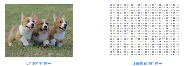
97.6. Image Processing#
Interestingly, SciPy integrates a large number of functions
and methods for image processing. Of course, a color image
is composed of RGB channels, which is actually a
multi-dimensional array. Therefore, the module for image
processing in SciPy,
scipy.ndimage, is actually a process for processing multi-dimensional
arrays, and you can complete a series of operations such as
convolution, filtering, and transformation.
Before formally understanding the
scipy.ndimage
module, we first import an example image of a raccoon using
the
face
method in the
scipy.misc
module.
scipy.misc
is a miscellaneous module that contains some methods that
cannot be accurately classified.
from scipy import misc

face = misc.face()
face
array([[[121, 112, 131],
        [138, 129, 148],
        [153, 144, 165],
        ...,
        [119, 126,  74],
        [131, 136,  82],
        [139, 144,  90]],

       [[ 89,  82, 100],
        [110, 103, 121],
        [130, 122, 143],
        ...,
        [118, 125,  71],
        [134, 141,  87],
        [146, 153,  99]],

       [[ 73,  66,  84],
        [ 94,  87, 105],
        [115, 108, 126],
        ...,
        [117, 126,  71],
        [133, 142,  87],
        [144, 153,  98]],

       ...,

       [[ 87, 106,  76],
        [ 94, 110,  81],
        [107, 124,  92],
        ...,
        [120, 158,  97],
        [119, 157,  96],
        [119, 158,  95]],

       [[ 85, 101,  72],
        [ 95, 111,  82],
        [112, 127,  96],
        ...,
        [121, 157,  96],
        [120, 156,  94],
        [120, 156,  94]],

       [[ 85, 101,  74],
        [ 97, 113,  84],
        [111, 126,  97],
        ...,
        [120, 156,  95],
        [119, 155,  93],
        [118, 154,  92]]], dtype=uint8)
By default,
face
is an RGB array of the image, and we can visualize and
restore it.
plt.imshow(face)
<matplotlib.image.AxesImage at 0x117390090>

Next, we try some image processing methods in
scipy.ndimage. For example, we perform Gaussian blur on the image.
from scipy import ndimage

plt.imshow(ndimage.gaussian_filter(face, sigma=5))
<matplotlib.image.AxesImage at 0x117391ed0>

Perform a rotation transformation on the image.
plt.imshow(ndimage.rotate(face, 45))
<matplotlib.image.AxesImage at 0x1174c8090>

Or perform a convolution operation on the image. First,
randomly define a convolution kernel
k, and then perform the convolution.
k = np.random.randn(2, 2, 3)
plt.imshow(ndimage.convolve(face, k))
<matplotlib.image.AxesImage at 0x1174c8150>

For more operations on multi-dimensional image arrays, please practice referring to the official documentation.
97.7. Optimization Methods#
Optimization is a branch of applied mathematics. Generally, we need to minimize (or maximize) an objective function, and the feasible solution found is also called the optimal solution. The idea of optimization is very common in the field of engineering applications. For example, machine learning algorithms all have an objective function, which we also call the loss function. And the process of finding the minimum value of the loss function is the optimization process. We may use optimization methods such as the least squares method, gradient descent method, Newton’s method, etc. to complete it.
The
scipy.optimize
module provided by SciPy contains a large number of
pre-written optimization methods. For example, the least
squares function
scipy.linalg.lstsq
we used above also has a very similar function
scipy.optimize.least_squares
in the
scipy.optimize
module. This function can solve non-linear least squares
problems.
The most commonly used function in the
scipy.optimize
module is
scipy.optimize.minimize, because a large number of optimization methods can be
selected just by specifying parameters. For example,
scipy.optimize.minimize(method="BFGS")
for the quasi-Newton method.
Next, we use the same data as in the demonstration of
scipy.linalg.lstsq
above and use the least squares method of
scipy.linalg.lstsq
to handle the least squares calculation process. It will be
a bit more troublesome here. First, define the fitting
function
func
and the residual function
err_func. In fact, we need to solve the minimum value of the
residual function.
def func(p, x):
    w0, w1 = p
    f = w0 + w1*x*x
    return f


def err_func(p, x, y):
    ret = func(p, x) - y
    return ret
from scipy.optimize import leastsq

p_init = np.random.randn(2)  # 生成 2 个随机数
x = np.array([1, 2.5, 3.5, 4, 5, 7, 8.5])
y = np.array([0.3, 1.1, 1.5, 2.0, 3.2, 6.6, 8.6])
# 使用 Scipy 提供的最小二乘法函数得到最佳拟合参数
parameters = leastsq(err_func, p_init, args=(x, y))
parameters[0]
array([0.20925826, 0.12013861])
Without accident, the results obtained here are exactly the
same as those obtained by
scipy.linalg.lstsq
above.
97.8. Signal Processing#
Signal Processing (English: Signal processing) refers to the process of processing signal representation, transformation, operation, etc. It is widely used in disciplines such as computer science, pharmaceutical analysis, and electronics. For decades, signal processing has played a key role in a wide range of fields such as voice and data communication, biomedical engineering, acoustics, sonar, radar, seismology, petroleum exploration, instrumentation, robotics, consumer electronics, and many others.
The related methods for signal processing in SciPy are in
the
scipy.signal
module, which is further divided into 13 subcategories such
as convolution, B-splines, filtering, window functions, peak
finding, spectral analysis, etc., with a total of more than
a hundred different functions and methods. Therefore, signal
processing is one of the very important modules in SciPy.
First, we try to generate some regular waveform diagrams, such as sawtooth waves, square waves, etc.
from scipy import signal

t = np.linspace(-1, 1, 100)

fig, axes = plt.subplots(1, 3, figsize=(12, 3))

axes[0].plot(t, signal.gausspulse(t, fc=5, bw=0.5))
axes[0].set_title("gausspulse")
t *= 5*np.pi
axes[1].plot(t, signal.sawtooth(t))
axes[1].set_title("chirp")
axes[2].plot(t, signal.square(t))
axes[2].set_title("gausspulse")
Text(0.5, 1.0, 'gausspulse')

Next, let’s try to apply several filtering functions. First, generate a set of waveform diagrams containing noise.
def f(t): return np.sin(np.pi*t) + 0.1*np.cos(7*np.pi*t+0.3) + \
    0.2 * np.cos(24*np.pi*t) + 0.3*np.cos(12*np.pi*t+0.5)


t = np.linspace(0, 4, 400)
plt.plot(t, f(t))
[<matplotlib.lines.Line2D at 0x1269ab790>]

Then, we use the median filtering function
scipy.signal.medfilt
and the Wiener filtering function
scipy.signal.wiener
in SciPy.
plt.plot(t, f(t))
plt.plot(t, signal.medfilt(f(t), kernel_size=55), linewidth=2, label="medfilt")
plt.plot(t, signal.wiener(f(t), mysize=55), linewidth=2, label="wiener")
plt.legend()
<matplotlib.legend.Legend at 0x126ee5490>

It can be seen from the above figure that the filtering effect is very obvious.
Regarding the usage of more functions in the
scipy.signal
module, a great deal of accumulation of professional
knowledge about signal processing is required. We will not
explain it here. You can read the official documentation
according to your own needs to learn.
97.9. Statistical Functions#
Statistical theory has wide applications, especially in the
interdisciplinary fields formed with computer science and
other fields, providing strong theoretical support for data
analysis, machine learning, etc. SciPy naturally has
relevant functions for statistical analysis, which are
concentrated in the
scipy.stats
module.
The
scipy.stats
module contains a large number of probability distribution
functions, mainly including continuous distributions,
discrete distributions, and multivariate distributions. In
addition, there are also multiple subcategories such as
summary statistics, frequency statistics, transformations,
and tests. It basically covers all aspects of statistical
applications.
Next, we will take the relatively representative continuous
random variable function of the normal distribution,
scipy.stats.norm, as an example for introduction. We will try to randomly
draw 1000 normal distribution samples using the
.rvs
method and plot a bar chart.
from scipy.stats import norm

plt.hist(norm.rvs(size=1000))
(array([  4.,  29.,  87., 172., 250., 208., 163.,  71.,  15.,   1.]),
 array([-3.03966428, -2.42019738, -1.80073047, -1.18126357, -0.56179666,
         0.05767024,  0.67713715,  1.29660406,  1.91607096,  2.53553787,
         3.15500477]),
 <BarContainer object of 10 artists>)

In addition to
norm.rvs
which returns random variables,
norm.pdf
returns the probability density function,
norm.cdf
returns the cumulative distribution function,
norm.sf
returns the survival function,
norm.ppf
returns the quantile function,
norm.isf
returns the inverse survival function,
norm.stats
returns the mean, variance, (Fisher) skewness, (Fisher)
kurtosis, and
norm.moment
returns the non-central moments of the distribution. For
these mentioned methods, they are common for most SciPy
continuous variable distribution functions (Cauchy
distribution, Poisson distribution, etc.).
For example, a normal distribution curve can be plotted based on the probability density function.
x = np.linspace(norm.ppf(0.01), norm.ppf(0.99), 1000)
plt.plot(x, norm.pdf(x))
[<matplotlib.lines.Line2D at 0x126fe4e10>]

In addition, the
scipy.stats
module also has many useful methods, such as returning a
summary of the data.
from scipy.stats import describe

describe(x)
DescribeResult(nobs=1000, minmax=(-2.3263478740408408, 2.3263478740408408), mean=0.0, variance=1.809385737250562, skewness=9.356107558947013e-17, kurtosis=-1.2000024000024)
describe
can return information such as the maximum value, minimum
value, mean, variance, etc. of a given array. The
scipy.stats
module involves relatively strong professionalism and has a
relatively high application threshold. You need to be
familiar with statistical theories to understand the
interpretations of the functions therein.
97.10. Sparse Matrix#
In numerical analysis, a matrix with most of its elements being zero is called a sparse matrix. Conversely, if most of the elements are non-zero, then the matrix is dense. Large sparse matrices often appear when solving linear models in the fields of science and engineering. However, computers often encounter many troubles when performing sparse matrix operations. Due to its own sparse characteristics, memory cost of sparse matrices can be greatly saved through compression. More importantly, due to their large size, standard algorithms often cannot operate on these sparse matrices.
Therefore, the
scipy.sparse
module in SciPy provides storage methods for sparse
matrices, and
scipy.sparse.linalg
contains processing methods specifically for sparse linear
algebra. In addition,
scipy.sparse.csgraph
also contains some theories of topological graphs of sparse
matrices.
There are roughly seven types of sparse matrix storage
methods in
scipy.sparse, namely:
csc_matrix
(compressed sparse column matrix),
csr_matrix
(compressed sparse row matrix),
bsr_matrix
(block sparse row matrix),
lil_matrix
(row-based linked list sparse matrix),
dok_matrix
(dictionary-based sparse matrix),
coo_matrix
(sparse matrix in coordinate format), and
dia_matrix
(diagonal sparse matrix).
Next, using a simple NumPy array as an example, convert it
to sparse matrix storage. First is the
csr_matrix
(compressed sparse row matrix).
from scipy.sparse import csr_matrix

array = np.array([[2, 0, 0, 3, 0, 0], [1, 0, 1, 0, 0, 2], [0, 0, 1, 2, 0, 0]])
csr = csr_matrix(array)
print(csr)
  (0, 0)	2
  (0, 3)	3
  (1, 0)	1
  (1, 2)	1
  (1, 5)	2
  (2, 2)	1
  (2, 3)	2
As can be seen, when storing a sparse matrix, the positions
of non-zero elements in the matrix are actually represented
in the form of coordinates. Next, try to store the same
array using the
csc_matrix
(compressed sparse column matrix).
from scipy.sparse import csc_matrix

csc = csc_matrix(array)
print(csc)
  (0, 0)	2
  (1, 0)	1
  (1, 2)	1
  (2, 2)	1
  (0, 3)	3
  (2, 3)	2
  (1, 5)	2
In fact, by comparison, it can be seen that the storage
orders of the two are different, one is row order and the
other is column order. The sparse matrix representation can
be converted to a dense matrix representation through
todense().
csc.todense()
matrix([[2, 0, 0, 3, 0, 0],
        [1, 0, 1, 0, 0, 2],
        [0, 0, 1, 2, 0, 0]])
Next, we compare the memory sizes consumed when storing sparse matrices and dense matrices. First, we generate a \(1000 \times 1000\) random matrix, and then replace the values less than 1 with 0 to artificially create a sparse matrix.
from scipy.stats import uniform

data = uniform.rvs(size=1000000, loc=0, scale=2).reshape(1000, 1000)
data[data < 1] = 0
data
array([[0.        , 1.71868732, 1.58826023, ..., 1.92015453, 1.95429687,
        0.        ],
       [1.98569154, 0.        , 1.85929614, ..., 0.        , 1.17994845,
        1.3283427 ],
       [1.78262258, 1.13269682, 0.        , ..., 0.        , 0.        ,
        1.97596699],
       ...,
       [0.        , 0.        , 0.        , ..., 1.53329049, 0.        ,
        0.        ],
       [0.        , 0.        , 0.        , ..., 1.73593538, 1.44965897,
        1.16125691],
       [1.94369028, 1.77482989, 1.35591931, ..., 0.        , 0.        ,
        0.        ]])
Next, we print the storage size consumed by this dense matrix in memory, with the unit of MB.
data.nbytes/(1024**2)
7.62939453125
Next, we store it as a sparse matrix and view the size in the same unit.
data_csr = csr_matrix(data)
data_csr.data.size/(1024**2)
0.4768686294555664
Without accident, the memory space consumed by storing in the sparse matrix format should be much less than that in the dense matrix storage method.
97.11. Summary#
In this chapter, we introduced a series of methods for scientific computing using SciPy. These include: constant modules, linear algebra, interpolation functions, image processing, optimization methods, signal processing, statistical functions, sparse matrices, etc. However, for this series of modules in SciPy, we only completed basic applications and exercises. Subsequently, you need to conduct in-depth learning and understanding of specific content based on your actual situation and in combination with the introduction in the official documentation.