
30. Implementation and Application of Density Clustering Method#
30.1. Introduction#
After mastering the partitioning clustering and hierarchical clustering methods, we also need to understand and learn a type of clustering method, namely density clustering. Density clustering divides the corresponding categories by evaluating the closeness of samples. In theory, it can find clusters of any shape and effectively avoid the interference of noise. In addition, like hierarchical clustering, density clustering does not need to declare in advance the number of categories to be clustered as in partitioning clustering.
30.2. Key Points#
DBSCAN Density Clustering Algorithm
-
Implementation of DBSCAN Clustering Algorithm
HDBSCAN Clustering Algorithm
30.3. Overview of Density Clustering Methods#
In the content of the previous class, we learned about hierarchical clustering methods and introduced the bottom-up, top-down, and more efficient BIRCH hierarchical clustering algorithms. Hierarchical clustering effectively avoids the trouble of having to specify the number of clustering categories in advance in partitioning clustering and facilitates us to obtain different clustering results as needed by generating a hierarchical tree structure.
However, hierarchical clustering has some inevitable congenital drawbacks. For example, like partitioning clustering methods, it cannot well approximate the clustering problem of non-convex data, which will be elaborated in detail below. Therefore, later, someone proposed the density clustering method.
Density clustering divides corresponding categories by evaluating the closeness of samples. In theory, it can find clusters of any shape, including non-convex data. In addition, density clustering also does not require prior knowledge of the number of clusters to be formed and can effectively identify noise points. Therefore, density clustering is also a very commonly used clustering algorithm.
30.4. DBSCAN Density Clustering Algorithm#
The most commonly used density clustering algorithm is the DBSCAN algorithm. DBSCAN is an abbreviation of Density-based spatial clustering of applications with noise, which literally means “density-based clustering method with noise”. This method was proposed by Martin Ester et al. in 1996.
Compared with other clustering methods, the significant advantage of DBSCAN is that it can discover clusters of various shapes and sizes in noisy data. Additionally, compared with partitioning clustering methods, DBSCAN does not require the number of clusters to be declared in advance, which is very similar to hierarchical clustering in this regard.
30.5. DBSCAN Clustering Principle#
As a typical density clustering method, the clustering principle of DBSCAN is of course related to density. Briefly speaking, DBSCAN generally assumes that the categories of samples can be determined by the degree of closeness of the sample distribution. So it first discovers points with high density, then gradually connects adjacent high-density points into a single area, and thus finds different categories (clusters).
Next, let’s use an example to illustrate the specific operation process of DBSCAN.
-
First, DBSCAN will draw a circle with each data point as the center and \(eps\) (\(\varepsilon\)-neighborhood) as the radius.
-
Then, DBSCAN will calculate how many other points are in the corresponding circle and use this number as the density value of the center data point.
-
Next, we need to determine the density threshold MinPts and classify data points (including themselves) with a density less than or greater than this density threshold as low-density or high-density points (core points) respectively.
-
If, at this time, a high-density point is within the circle range of another high-density point, we connect these two points.
-
After that, if a low-density point is also within the circle range of a high-density point, it is also connected to the nearest high-density point and is called a border point.
Finally, all the data points that can be connected together form a clustering category. And some points that cannot be connected are defined as outliers. Next, we will elaborate on this process in detail according to a diagram.
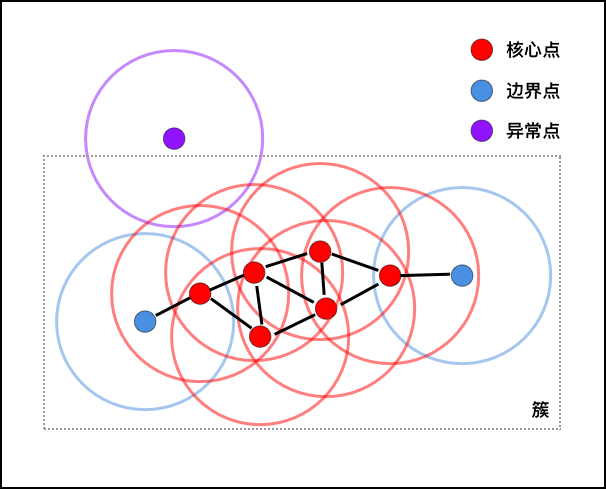
As shown in the figure above, assuming that we specify the
density threshold
MinPts
                      =
                      4
, then the red points in the figure are core points because
there are at least 4 points (including themselves) in their
\(\varepsilon\)-neighborhood. Since they are mutually reachable, they form
a cluster. The blue points in the figure are not core
points, but they are within the circles of the core points,
so they also belong to the same cluster, that is, border
points. The purple points are neither core points nor border
points, so they are called outliers.
The above is the entire process of DBSCAN clustering. It seems quite simple and clear, right!
30.7. Python Implementation of DBSCAN Clustering Algorithm#
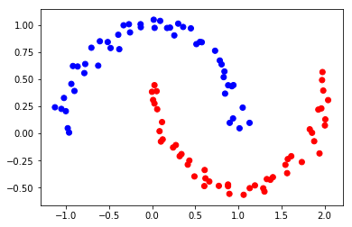
Before implementing the DBSCAN clustering process, we also
need to generate a set of sample data first. This time,
instead of generating clustered data, we generate
crescent-shaped data chunks. Here, the
make_moons
method is used.
from sklearn import datasets

noisy_moons, _ = datasets.make_moons(
    n_samples=100, noise=0.05, random_state=10
)  # 生成 100 个样本并添加噪声
noisy_moons[:5]
array([[ 0.2554364 ,  0.90420806],
       [ 0.55299636,  0.84445141],
       [-0.90343862,  0.39161309],
       [-0.62792219,  0.62502915],
       [ 0.60777269, -0.33777687]])
from matplotlib import pyplot as plt

%matplotlib inline

plt.scatter(noisy_moons[:, 0], noisy_moons[:, 1])
<matplotlib.collections.PathCollection at 0x130bcbc10>

As can be seen from the above figure, although the distribution of data points is rather strange, it is obvious to the naked eye that there are two categories, similar to the following figure:
At this time, we try to use K-Means in partitioning clustering and BIRCH in hierarchical clustering to attempt to cluster the above dataset. As we all know, these two methods are representatives of partitioning and hierarchical clustering methods. Here, for convenience, we directly use scikit-learn to implement them.
from sklearn.cluster import KMeans, Birch

kmeans_c = KMeans(n_clusters=2, n_init="auto").fit_predict(noisy_moons)
birch_c = Birch(n_clusters=2).fit_predict(noisy_moons)

fig, axes = plt.subplots(nrows=1, ncols=2, figsize=(15, 5))
axes[0].scatter(noisy_moons[:, 0], noisy_moons[:, 1], c=kmeans_c, cmap="bwr")
axes[1].scatter(noisy_moons[:, 0], noisy_moons[:, 1], c=birch_c, cmap="bwr")
axes[0].set_xlabel("K-Means")
axes[1].set_xlabel("BIRCH")
Text(0.5, 0, 'BIRCH')

Was the above result a big disappointment to you? The K-Means and BIRCH methods, which performed very well in the previous experiments, actually failed to correctly cluster the above sample data. In fact, in the face of such concave-shaped datasets, partitioning and hierarchical clustering methods often cannot correctly cluster, and this is when density clustering methods come into play.
Next, we will try to implement the DBSCAN density clustering algorithm using Python. I wonder if you still remember the principle of DBSCAN clustering. If it’s a bit fuzzy, go back to the previous section and review it again. Because the implementation process of the algorithm is actually the process of DBSCAN clustering.
First, we implement a
search_neighbors()
function, whose purpose is to find the reachable data points
around the core points. Among them, the Euclidean distance
is used to calculate the distance.
import numpy as np


def euclidean_distance(a, b):
    """
    参数:
    a -- 数组 a
    b -- 数组 b

    返回:
    dist -- a, b 间欧式距离
    """
    # 欧式距离
    x = float(a[0]) - float(b[0])
    x = x * x
    y = float(a[1]) - float(b[1])
    y = y * y
    dist = round(np.sqrt(x + y), 2)
    return dist
def search_neighbors(D, P, eps):
    """
    参数:
    D -- 数据集(二维数组)
    P -- 核心点
    eps -- eps 邻域

    返回:
    neighbors -- 核心点在 eps 范围内的邻居
    """
    # 找出数据集中距核心点 P 在 eps 范围内的邻近点
    neighbors = []
    for Pn in range(0, len(D)):
        # 距离判断是否在 eps 范围内
        if euclidean_distance(D[P], D[Pn]) < eps:
            neighbors.append(Pn)

    return neighbors
Next, we implement the main code of DBSCAN:
def dbscan_cluster(D, eps, MinPts):
    """
    参数:
    D -- 数据集(二维数组)
    eps -- eps 邻域
    MinPts -- 密度阀值

    返回:
    labels -- 聚类标签
    """
    # DBSCAN 密度聚类算法
    labels = [0] * len(D)  # 初始化数据集中的数据类别全部为 0
    C = 0
    # 选择 P 作为核心点
    for P in range(0, len(D)):
        # 选择类别为 0 的点作为中心
        if not (labels[P] == 0):
            continue

        # 搜寻该数据点在 eps 圆中的邻居
        Neighbors = search_neighbors(D, P, eps)

        # 标记噪声点为 -1
        if len(Neighbors) < MinPts:
            labels[P] = -1

        # 非噪声点作为新类别中心
        else:
            C += 1  # 原类别 +1 作为新类别的标签
            labels[P] = C  # 将非噪声点设定为新类别

            # 开始检查 P 在 eps 圆中邻居的可达性
            for i, n in enumerate(Neighbors):
                Pn = Neighbors[i]  # 从 P 的邻居中取 1 个点

                # P 的邻居,设定为一样的类别
                if labels[Pn] == 0:
                    labels[Pn] = C

                    # 进一步搜索 P 的邻居的邻居
                    PnNeighbors = search_neighbors(D, Pn, eps)
                    if len(PnNeighbors) >= MinPts:  # 如果满足密度阈值要求则连通
                        Neighbors += PnNeighbors

                # 如果该点曾被标记为噪声点, 则重新连接到类别中
                elif labels[Pn] == -1:
                    labels[Pn] = C

    return labels
Now, we use the DBSCAN algorithm to cluster the above
crescent-shaped sample data to obtain the clustering labels.
Here, we set the value of the
\(\varepsilon\)-neighborhood to
0.5, and the density threshold
MinPts
                      =
                      5
, that is, at least 5 other points within a circle with a
radius of
0.5
can be regarded as core points.
dbscan_c = dbscan_cluster(noisy_moons, eps=0.5, MinPts=5)
np.array(dbscan_c)  # 显示聚类标签
array([1, 1, 1, 1, 2, 1, 2, 1, 1, 2, 1, 1, 2, 2, 2, 2, 2, 1, 2, 1, 2, 2,
       2, 1, 2, 2, 1, 2, 1, 2, 1, 1, 2, 2, 1, 1, 1, 1, 1, 1, 1, 1, 2, 2,
       1, 2, 1, 2, 2, 1, 2, 2, 2, 2, 1, 1, 2, 2, 2, 2, 1, 1, 2, 2, 1, 1,
       2, 2, 1, 2, 1, 2, 1, 2, 1, 1, 2, 2, 2, 2, 1, 2, 2, 1, 2, 2, 1, 1,
       1, 1, 1, 2, 1, 1, 2, 2, 1, 2, 1, 1])
According to the clustering labels obtained by the DBSCAN algorithm, recolour the scatter plot to view the clustering effect.
plt.scatter(noisy_moons[:, 0], noisy_moons[:, 1], c=dbscan_c, cmap="bwr")
<matplotlib.collections.PathCollection at 0x136bdd2a0>

As shown in the figure above, the DBSCAN clustering results meet our psychological expectations and at the same time make up for the deficiencies of partitioning and hierarchical clustering.
30.8. Implementation of DBSCAN Clustering Algorithm in scikit-learn#
We have already implemented the DBSCAN clustering algorithm using Python. In fact, scikit-learn also provides APIs related to DBSCAN clustering. Let’s take a look at how to use them:
sklearn.cluster.DBSCAN(eps=0.5, min_samples=5, metric='euclidean', metric_params=None, algorithm='auto', leaf_size=30, p=None, n_jobs=1)
Among them, the main parameters are:
eps: The value of the epsilon-neighborhood.
-
min_samples: The value of the density threshold MinPts.
-
metric: The distance metric method, with the default being the Euclidean distance.
-
algorithm: The method for solving the nearest neighbor algorithm: auto, ball_tree, kd_tree, brute are available options.
Meanwhile, complete the clustering for the sample data.
from sklearn.cluster import DBSCAN

dbscan_sk = DBSCAN(eps=0.5, min_samples=5, metric="euclidean")
dbscan_sk_c = dbscan_sk.fit_predict(noisy_moons)
dbscan_sk_c
array([0, 0, 0, 0, 1, 0, 1, 0, 0, 1, 0, 0, 1, 1, 1, 1, 1, 0, 1, 0, 1, 1,
       1, 0, 1, 1, 0, 1, 0, 1, 0, 0, 1, 1, 0, 0, 0, 0, 0, 0, 0, 0, 1, 1,
       0, 1, 0, 1, 1, 0, 1, 1, 1, 1, 0, 0, 1, 1, 1, 1, 0, 0, 1, 1, 0, 0,
       1, 1, 0, 1, 0, 1, 0, 1, 0, 0, 1, 1, 1, 1, 0, 1, 1, 0, 1, 1, 0, 0,
       0, 0, 0, 1, 0, 0, 1, 1, 0, 1, 0, 0])
According to the obtained clustering labels, recolour the scatter plot to view the clustering effect.
plt.scatter(noisy_moons[:, 0], noisy_moons[:, 1], c=dbscan_sk_c, cmap="bwr")
<matplotlib.collections.PathCollection at 0x136c74a30>
It can be seen that the above figure is exactly the same as the calculation result of the algorithm manually implemented by us using Python.
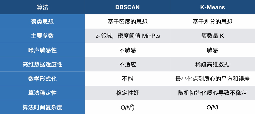
Finally, let’s compare the DBSCAN and K-Means methods together again.
30.9. HDBSCAN Clustering Algorithm#
The HDBSCAN clustering algorithm was proposed by Campello, Moulavi, and Sander in 2013. This is a relatively new clustering method, and its full English name is: Density-Based Clustering Based on Hierarchical Density Estimates. If you are careful enough, you will find that the extra ‘H’ in HDBSCAN compared to the DBSCAN algorithm is actually ‘Hierarchical’, which is exactly the English word for hierarchical clustering method.
And the literal Chinese translation of HDBSCAN is: Density clustering method based on hierarchical density estimation.
Before discussing HDBSCAN, let’s first talk about a major drawback of the DBSCAN algorithm, which is its parameter sensitivity.
DBSCAN is greatly affected by parameter changes. Especially when the data distribution density is uneven, if we set eps to a small value, then the categories with relatively low density will be further divided into multiple subcategories. Similarly, when the eps value is set to be large, it will cause the categories that are close in distance and have a large density to be merged into one cluster. This also reflects the instability of DBSCAN.
HDBSCAN improves the instability of DBSCAN by combining the characteristics of hierarchical clustering. Therefore, the clustering process is changed to two steps:
-
Generate the original clusters. This stage is similar to the first stage of the DBSCAN algorithm, determining the core points, generating the original clusters, and effectively identifying the noise points.
-
Merge the original clusters. In this stage, the idea of hierarchical clustering is used to merge the original clusters, reducing the sensitivity of the clustering results to the input parameters. Since this method does not require testing and judging each object, it also reduces the time complexity.
30.10. Comparison between DBSCAN and HDBSCAN Clustering#
Next, let’s take a look at how HDBSCAN specifically works and what its advantages are compared to DBSCAN?
First, we regenerate a set of sample data:
moons, _ = datasets.make_moons(n_samples=50, noise=0.05, random_state=10)
blobs, _ = datasets.make_blobs(
    n_samples=50, centers=[(-0.25, 3.25), (3, 3.5)], cluster_std=0.6, random_state=10
)

noisy_moons_blobs = np.vstack([moons, blobs])
plt.scatter(noisy_moons_blobs[:, 0], noisy_moons_blobs[:, 1], color="b")
<matplotlib.collections.PathCollection at 0x136d00490>

As shown in the figure above, this dataset contains two cluster-shaped data and a set of crescent-shaped data. First, we use the DBSCAN algorithm to cluster it and see what happens:
dbscan_sk_c = dbscan_sk.fit_predict(noisy_moons_blobs)
dbscan_sk_c
array([ 0,  1,  0,  0,  0,  1,  1,  0,  1,  1,  0,  1,  0,  0,  1,  1,  0,
        0,  1,  0,  1,  1,  0,  0,  0,  1,  1,  1,  1,  1,  1,  1,  0,  0,
        1,  1,  0,  1,  0,  0,  0,  1,  0,  0,  0,  0,  1,  1,  0,  1, -1,
        2, -1,  2,  2, -1,  3,  3,  3,  2,  3, -1,  3,  2,  3,  2, -1,  2,
        2, -1,  2,  3,  3,  2, -1, -1,  3, -1,  3,  2, -1,  3, -1,  3,  2,
        3,  3, -1,  2, -1, -1,  2,  3,  3, -1, -1, -1,  3,  3,  3])
plt.scatter(
    noisy_moons_blobs[:, 0], noisy_moons_blobs[:, 1], c=dbscan_sk_c, cmap="cool"
)
<matplotlib.collections.PathCollection at 0x136d6d420>

By observation, the DBSCAN algorithm clusters the
noisy_moons_blobs
dataset into 4 categories and marks the outliers around the
cluster-shaped data.
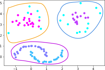
In fact, by visual inspection, the optimal clustering for
the
noisy_moons_blobs
dataset should be 3 categories. Although the crescent-shaped
data above was divided into 2 categories, it is obvious here
that the crescent-shaped data is regarded as one category
and is well distinguished from the cluster-shaped data, that
is, as shown in the following figure.
So, can the DBSCAN algorithm achieve this? We can give it a
try by increasing the
eps
parameter:
dbscan_sk = DBSCAN(eps=1, min_samples=5, metric="euclidean")
dbscan_sk_c = dbscan_sk.fit_predict(noisy_moons_blobs)
plt.scatter(
    noisy_moons_blobs[:, 0], noisy_moons_blobs[:, 1], c=dbscan_sk_c, cmap="cool"
)
<matplotlib.collections.PathCollection at 0x136db55d0>

By increasing the
eps
parameter from 0.5 to 1, we successfully clustered the
dataset into 3 categories and the noise points disappeared.
Of course, for such a small dataset in this article, perhaps
it can be completed by adjusting the parameters once.
However, in the face of real and complex datasets, it is
often necessary to continuously adjust the
eps
and
min_samples
parameters. The workload is not only huge, but also may not
achieve the desired clustering effect.
Next, we try to solve this problem at once with HDBSCAN.
Currently, the HDBSCAN algorithm is not included in scikit - learn. However, the complete implementation of the HDBSCAN algorithm is available in the scikit - learn - contrib branch. Here, we first need to install HDBSCAN using the following command.
{note}
pip install hdbscan
After installing and importing the module, parameters need
to be specified. The most important parameter in HDBSCAN is
min_cluster_size, which is used to determine the minimum number of samples
required to form a cluster. The second important parameter
is
min_samples. Briefly speaking, the larger the
min_samples
value, the more conservative the clustering effect, that is,
more points will be declared as noise.
Next, we directly use the default parameters of HDBSCAN
(min_cluster_size
=
5,
min_samples
                      =
                      None
) to complete the clustering process for the
noisy_moons_blobs
dataset.
import hdbscan

# gen_min_span_tree 参数为下文绘图做准备
hdbscan_m = hdbscan.HDBSCAN(gen_min_span_tree=True)
hdbscan_m_c = hdbscan_m.fit_predict(noisy_moons_blobs)

plt.scatter(
    noisy_moons_blobs[:, 0], noisy_moons_blobs[:, 1], c=hdbscan_m_c, cmap="winter"
)
<matplotlib.collections.PathCollection at 0x13788d150>

As can be seen, there are no
eps
and
MinPts
parameters in HDBSCAN. We only need to simply specify the
minimum number of samples to form clusters for adjustment to
complete the clustering, and the clustering effect is very
good.
30.11. HDBSCAN Algorithm Process [Optional]#
Next, we will analyze the clustering process of the HDBSCAN algorithm. Since it involves knowledge of graph theory, this part is for optional study and can be understood according to your own situation.
First of all, we need to clarify several definitions.
Core distance \(core_k(x)\): The distance between the current point and its \(k\)-th nearest point, usually using the Euclidean distance.
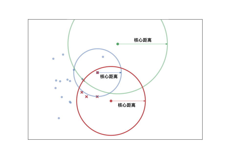
Mutual reachability distance \(d_{\mathrm{mreach-}k}(a,b)\): The distance from a core point to an adjacent core point, usually using the Euclidean distance.
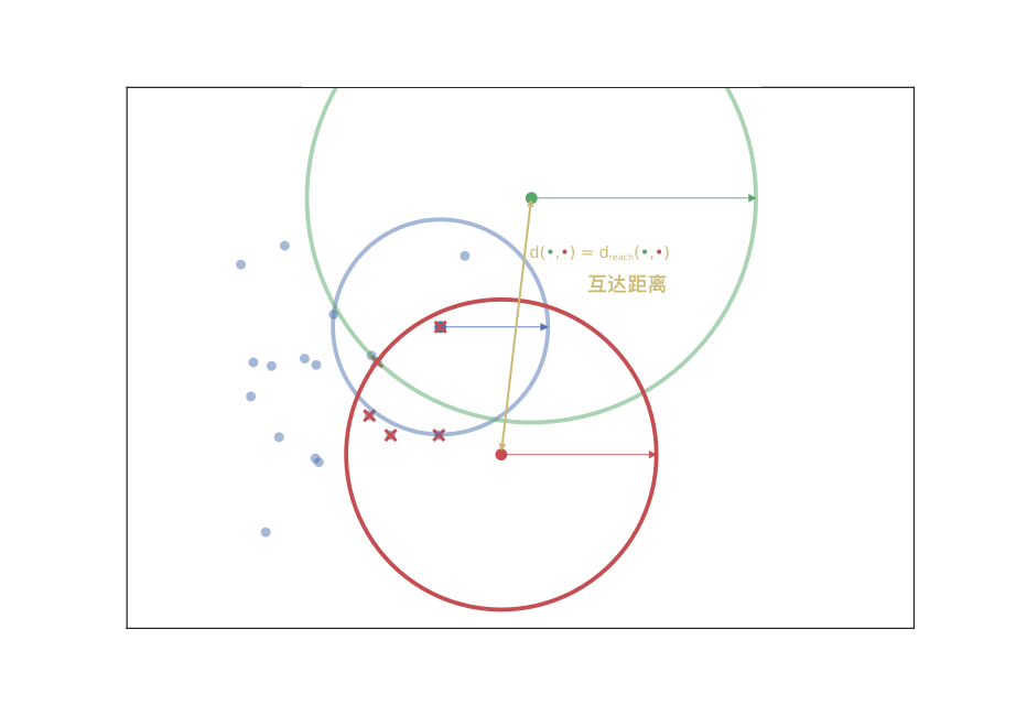
Now, we have a new measure of mutual reachability between data points, and then we start to find the noise points in the dense data. Of course, the dense areas are relative, and different clusters may have different densities. Conceptually, what we need to do is: draw a weighted graph for the data, with data points as vertices, and the weight corresponding to the edge between any two points is equal to the mutual reachability distance between the two points.
Thus, we can assume that there is a threshold \(\varepsilon\), and the edges with weights greater than \(\varepsilon\) are deleted. As the threshold changes from large to small, the connectivity of the entire graph will change. If each connected region is regarded as a cluster, a hierarchical clustering result that changes with \(\varepsilon\) can be obtained.
The simplest implementation method is to perform a connectivity judgment and update on the graph every time a threshold is set. However, practice has proved that the efficiency of such execution is too low. Fortunately, graph theory provides a means called the minimum spanning tree of the graph.
The definition of a spanning tree is as follows: for a data graph with \(n\) vertices, at least \(n - 1\) edges are required to connect these \(n\) vertices. The subgraph composed of these \(n - 1\) edges is called the spanning tree of the original graph.
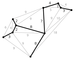
When the edges in the graph have weights, there will always be a spanning tree whose sum of edge weights is less than or equal to the sum of edge weights of other spanning trees. This is the minimum spanning subtree [the thick solid lines in the above figure].
Generally, we can construct the minimum spanning tree very efficiently through Prim’s algorithm. Of course, it is more ideal to use Boruvka’s algorithm to find the minimum spanning tree. The following figure is an animation of Boruvka’s algorithm finding the minimum spanning tree. The details of the algorithm will not be elaborated here.
Next, we use the
minimum_spanning_tree_.plot()
method provided by hdbscan to plot the minimum spanning
subtree when the HDBSCAN algorithm clusters the
noisy_moons_blobs
dataset.
plt.figure(figsize=(15, 8))
hdbscan_m.minimum_spanning_tree_.plot(
    edge_cmap="viridis", edge_alpha=0.4, node_size=90, edge_linewidth=3
)
<Axes: >

The above figure shows the minimum spanning tree of the
noisy_moons_blobs
dataset, where the colors correspond to the mutual
reachability distances (weights) between points.
Once we have the minimum spanning tree, we can construct the
cluster hierarchy. This process is very simple and is the
bottom-up hierarchical clustering process learned in the
previous hierarchical clustering. Similarly, we can directly
output the final hierarchical binary tree using the
single_linkage_tree_.plot()
method provided by hdbscan.
plt.figure(figsize=(15, 8))
hdbscan_m.single_linkage_tree_.plot(cmap="viridis", colorbar=True)
<Axes: ylabel='distance'>

In the figure, the length of the vertical lines corresponds to the distance, and the colors correspond to the cluster density.
Next, we can extract the clusters of the final clustering by pruning the binary tree. Here, we need to involve a new concept, the \(\lambda\)-index of the clusters:
At this time, we can plot the pruned hierarchical binary
tree using the
condensed_tree_.plot()
method provided by hdbscan.
plt.figure(figsize=(15, 8))
hdbscan_m.condensed_tree_.plot()
<Axes: ylabel='$\\lambda$ value'>

The vertical axis changes from the mutual reachability distance to the \(\lambda\)-index.
In fact, when each point is split, there are generally two cases: the current cluster is split into two sub-clusters, or the current cluster is split into a large cluster and several discrete points. Thus:
-
\(\lambda_{\mathrm{birth}}\) refers to the \(\lambda\) value when a cluster is formed.
-
\(\lambda_{\mathrm{death}}\) refers to the \(\lambda\) value when a cluster is split into two sub-clusters.
-
\(\lambda_{\mathrm{p}}\) refers to the \(\lambda\) value when point \(p\) separates from the cluster.
We hope that the stability of the cluster during splitting is as strong as possible. Thus, we can define an index to measure the stability of the cluster:
Therefore, during the splitting process of a cluster, if the sum of the stabilities of the two sub-clusters formed by the splitting is greater than that of the cluster, then we support this splitting; otherwise, we discard this splitting. In this way, we can traverse from the leaf nodes to the root node bottom-up to select the required clusters.
Similarly, we can use the
condensed_tree_.plot(select_clusters=True)
method provided by hdbscan to select clusters that meet the
stability characteristics.
plt.figure(figsize=(15, 8))
hdbscan_m.condensed_tree_.plot(select_clusters=True)
<Axes: ylabel='$\\lambda$ value'>

As shown in the figure above, the stable clustering clusters that finally meet the requirements are circled in red. The above is the principle process of HDBSCAN clustering.
30.12. Summary#
In this experiment, we mainly learned about the advantages of the DBSCAN density clustering method compared with hierarchical and partitioning clustering methods, and studied its principle and Python implementation process. In addition, we also learned about the relatively advanced HDBSCAN density clustering method and explained its clustering principle process. We suggest that you focus on mastering the principle and implementation of the DBSCAN algorithm and learn to use the HDBSCAN algorithm. Since the theory of HDBSCAN involves some graph theory knowledge, it is not required for everyone to master.
Related Links