Pro Membership

Pro Membership is a membership plan created by the author to maintain and update this tutorial. You can get more benefits and services, click to view details.

92. NumPy Numerical Computing Basics

92.1. Introduction

If you use the Python language for scientific computing, then you will definitely come into contact with NumPy. NumPy is an extension library for numerical computing that supports the Python language. It has powerful capabilities for processing multi-dimensional arrays and matrix operations. In addition, NumPy also has a large number of built-in functions to facilitate you to quickly build mathematical models.

92.2. Key Points

• Numerical types and multi-dimensional arrays

• Array operations and random sampling

• Mathematical functions and algebraic operations

• Array indexing and other usages

NumPy stands for Numerical Python, which means it is a third-party library for Python’s numerical computing. The feature of NumPy is that it expands the built-in array type in Python, supports higher-dimensional array and matrix operations, and has a richer set of mathematical functions.

NumPy is one of the most important libraries in Scipy.org. It is also used as the core computing library by third-party libraries such as Pandas and Matplotlib that we are familiar with. When you install these libraries separately, you will find that NumPy is installed as a dependency at the same time.

92.3. NumPy Array Types

Let’s first understand the data types supported by NumPy. The numerical types natively supported by Python are int (integer, long long integer existed in Python 2), float (floating point), bool (boolean), and complex (complex number).

NumPy supports a richer set of numerical types than Python itself, which are detailed as follows:

Type	Explanation
bool	Boolean type, 1 byte, with values True or False.
int	Integer type, usually int64 or int32.
intc	Same as int in C, usually int32 or int64.
intp	Used for indexing, usually int32 or int64.
int8	Byte (from -128 to 127)
int16	Integer (from -32768 to 32767)
int32	Integer (from -2147483648 to 2147483647)
int64	Integer (from -9223372036854775808 to 9223372036854775807)
uint8	Unsigned integer (from 0 to 255)
uint16	Unsigned integer (from 0 to 65535)
uint32	Unsigned integer (from 0 to 4294967295)
uint64	Unsigned integer (from 0 to 18446744073709551615)
float	Shorthand for float64.
float16	Half-precision floating point, 5-bit exponent, 10-bit mantissa
float32	Single-precision floating point, 8-bit exponent, 23-bit mantissa
float64	Double-precision floating point, 11-bit exponent, 52-bit mantissa
complex	Shorthand for complex128.
complex64	Complex number, represented by two 32-bit floating points.
complex128	Complex number, represented by two 64-bit floating points.

In NumPy, these numerical types mentioned above are all attributed to instances of the dtype (data-type) object. We can use numpy.dtype(object, align, copy) to specify the numerical type. And inside an array, we can use the dtype= parameter.

Next, let’s start learning NumPy. First, we need to import NumPy.

import numpy as np  # 导入 NumPy 模块

a = np.array([1.1, 2.2, 3.3], dtype=np.float64)  # 指定 1 维数组的数值类型为 float64
a, a.dtype  # 查看 a 及 dtype 类型

(array([1.1, 2.2, 3.3]), dtype('float64'))

You can use the .astype() method to convert between different numerical types.

a.astype(int).dtype  # 将 a 的数值类型从 float64 转换为 int，并查看 dtype 类型

dtype('int64')

92.4. NumPy Array Generation

Among Python built-in objects, there are three forms of arrays:

• Lists: [1, 2, 3]

• Tuples: (1, 2, 3, 4, 5)

• Dictionaries: {A:1, B:2}

Among them, tuples are similar to lists, but the difference is that the elements of tuples cannot be modified. And dictionaries are composed of keys and values. The Python standard classes have limitations in handling arrays, which are limited to one dimension and only provide a small number of functions. And one of the most core and important features of NumPy is the ndarray multi-dimensional array object. Different from Python’s standard classes, it has the ability to handle high-dimensional arrays, which is also an essential feature in the process of numerical calculation.

In NumPy, the ndarray class has six parameters, which are:

• shape: The shape of the array.

• dtype: The data type.

• buffer: The object exposes a buffer interface.

• offset: The offset of the array data.

• strides: The data strides.

• order: {'C', 'F'}, the row-major or column-major ordering.

Next, let’s learn about some methods for creating NumPy multi-dimensional arrays. In NumPy, we mainly create arrays through the following five ways, which are:

• Convert from Python array structures such as lists, tuples, etc.

• Use native NumPy methods such as np.arange, np.ones, np.zeros, etc.

• Read arrays from storage.

• Create arrays from raw bytes by using strings or buffers.

• Use special functions such as random.

92.4.1. List or Tuple Conversion

In NumPy, we use numpy.array to convert a list or tuple into an ndarray array. The method is as follows:

numpy.array(object, dtype=None, copy=True, order=None, subok=False, ndmin=0)

Among them, the parameters are as follows:

• object: list, tuple, etc.

• dtype: data type. If not given, the type is the minimum type required for the object to be saved.

• copy: boolean, default True, indicating to copy the object.

• order: order.

• subok: boolean, indicating whether subclasses are passed.

• ndmin: the minimum number of dimensions that the generated array should have.

Next, create an ndarray array from a list.

np.array([[1, 2, 3], [4, 5, 6]])

array([[1, 2, 3],
       [4, 5, 6]])

Or lists and tuples.

np.array([(1, 2), (3, 4), (5, 6)])

array([[1, 2],
       [3, 4],
       [5, 6]])

92.4.2. Creation with the arange method

In addition to directly creating ndarray using the array method, there are also some methods in NumPy to create multi-dimensional arrays with certain regularities. First, let’s take a look at arange(). The function of arange() is to create a series of evenly spaced values within a given interval. The method is as follows:

numpy.arange(start, stop, step, dtype=None)

You need to first set the interval [start, stop) where the values are located. This is a half-open and half-closed interval. Then, set the step to define the interval between values. The final optional parameter dtype can be used to set the value type of the returned ndarray.

# 在区间 [3, 7) 中以 0.5 为步长新建数组
np.arange(3, 7, 0.5, dtype='float32')

array([3. , 3.5, 4. , 4.5, 5. , 5.5, 6. , 6.5], dtype=float32)

92.4.3. Creation with the linspace method

The linspace method can also create arrays with regular numerical values, similar to the arange method. linspace is used to return evenly spaced values within a specified interval. The method is as follows:

numpy.linspace(start, stop, num=50, endpoint=True, retstep=False, dtype=None)

• start: The starting value of the sequence.

• stop: The ending value of the sequence.

• num: The number of samples to generate. The default value is 50.

• endpoint: A boolean value. If true, the last sample is included in the sequence.

• retstep: A boolean value. If true, return the spacing.

• dtype: The type of the array.

np.linspace(0, 10, 10, endpoint=True)

array([ 0.        ,  1.11111111,  2.22222222,  3.33333333,  4.44444444,
        5.55555556,  6.66666667,  7.77777778,  8.88888889, 10.        ])

Change the endpoint parameter to False and see the difference:

np.linspace(0, 10, 10, endpoint=False)

array([0., 1., 2., 3., 4., 5., 6., 7., 8., 9.])

92.4.4. Creation with the ones Method

numpy.ones is used to quickly create multi-dimensional arrays with all elements being 1. The method is as follows:

numpy.ones(shape, dtype=None, order='C')

Among them:

• shape: Used to specify the shape of the array, such as (1, 2) or 3.

• dtype: The data type.

• order: {'C', 'F'}, storing the array row-wise or column-wise.

np.ones((2, 3))

array([[1., 1., 1.],
       [1., 1., 1.]])

92.4.5. Creation with the zeros Method

The zeros method is very similar to the ones method above. The difference is that here all elements are filled with 0. The zeros method is consistent with the ones method.

numpy.zeros(shape, dtype=None, order='C')

Among them:

• shape: Used to specify the shape of the array, such as (1, 2) or 3.

• dtype: Data type.

• order: {'C', 'F'}, store the array row-wise or column-wise.

np.zeros((3, 2))

array([[0., 0.],
       [0., 0.],
       [0., 0.]])

92.4.6. Creation with the eye method

numpy.eye is used to create a two-dimensional array where the values on the k-diagonal are 1 and all other values are 0. The method is as follows:

numpy.eye(N, M=None, k=0, dtype=<type 'float'>)

Where:

• N: The number of rows of the output array.

• M: The number of columns of the output array.

• k: The diagonal index: 0 (default) refers to the main diagonal, positive values refer to the upper diagonals, and negative values refer to the lower diagonals.

np.eye(5, 4, 3)

array([[0., 0., 0., 1.],
       [0., 0., 0., 0.],
       [0., 0., 0., 0.],
       [0., 0., 0., 0.],
       [0., 0., 0., 0.]])

92.4.7. Create from Known Data

We can also create ndarray from known data files and functions. NumPy provides the following five methods:

• frombuffer(buffer): Convert a buffer into a 1-D array.

• fromfile(file, dtype, count, sep): Construct a multi-dimensional array from a text or binary file.

• fromfunction(function, shape): Create a multi-dimensional array by the function’s return values.

• fromiter(iterable, dtype, count): Create a 1-D array from an iterable object.

• fromstring(string, dtype, count, sep): Create a 1-D array from a string.

np.fromfunction(lambda a, b: a + b, (5, 4))

array([[0., 1., 2., 3.],
       [1., 2., 3., 4.],
       [2., 3., 4., 5.],
       [3., 4., 5., 6.],
       [4., 5., 6., 7.]])

92.4.8. ndarray Array Attributes

First, we create an ndarray array. First, create a and arbitrarily set it as a 2-D array.

a = np.array([[1, 2, 3], [4, 5, 6], [7, 8, 9]])
a  # 查看 a 的值

array([[1, 2, 3],
       [4, 5, 6],
       [7, 8, 9]])

ndarray.T is used for transposing an array, which is the same as .transpose().

a.T

array([[1, 4, 7],
       [2, 5, 8],
       [3, 6, 9]])

ndarray.dtype is used to output the data type of the elements contained in the array.

a.dtype

dtype('int64')

ndarray.imag is used to output the imaginary part of the elements contained in the array.

a.imag

array([[0, 0, 0],
       [0, 0, 0],
       [0, 0, 0]])

ndarray.real is used to output the real part of the elements contained in the array.

a.real

array([[1, 2, 3],
       [4, 5, 6],
       [7, 8, 9]])

ndarray.size is used to output the total number of elements contained in the array.

a.size

9

ndarray.itemsize outputs the number of bytes of one array element.

a.itemsize

8

ndarray.nbytes is used to output the total number of bytes of the array elements.

a.nbytes

72

ndarray.ndim is used to output the number of dimensions of the array.

a.ndim

2

ndarray.shape is used to output the shape of the array.

a.shape

(3, 3)

ndarray.strides outputs the byte array of steps in each dimension when traversing the array.

a.strides

(24, 8)

92.5. Array Dimensions and Shapes

Previously, we have introduced the types of NumPy arrays and common generation methods. Before continuing to learn more, it is necessary to clarify an important issue, that is, the dimensions and shapes of NumPy arrays.

NumPy arrays are also known as ndarray multi-dimensional arrays, so n can increase sequentially from 1 dimension. In the following figure, we show examples of NumPy arrays from 1 to 3 dimensions.

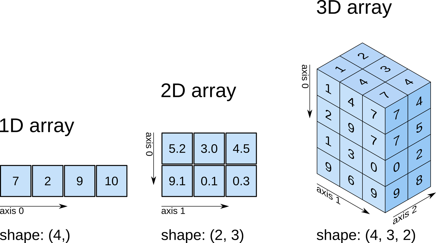
1D arrays can be regarded as vectors in mathematics, 2D arrays can be regarded as matrices, and 3D arrays are data cubes.

Next, we try to generate the example arrays as shown in the figure. Some of the values in the three-dimensional array cannot be obtained from the figure, and we replace them all with 1.

one = np.array([7, 2, 9, 10])
two = np.array([[5.2, 3.0, 4.5],
                [9.1, 0.1, 0.3]])
three = np.array([[[1, 1], [1, 1], [1, 1]],
                  [[1, 1], [1, 1], [1, 1]],
                  [[1, 1], [1, 1], [1, 1]],
                  [[1, 1], [1, 1], [1, 1]]])

Next, we use the .shape attribute to view the shape of the NumPy array.

one.shape, two.shape, three.shape

((4,), (2, 3), (4, 3, 2))

You can find the pattern that the shape obtained by .shape is actually the number of elements of the array on each axis, and the length of .shape indicates the dimension of the array.

92.6. Basic Array Operations

So far, we have learned how to use NumPy to create various ndarrays, as well as the concepts of array shape and dimension. Next, we will learn various fancy operation techniques for ndarrays.

92.6.1. Reshape

reshape can change the shape of an array without changing its data. Among them, numpy.reshape() is equivalent to ndarray.reshape(). The reshape method is very simple:

numpy.reshape(a, newshape)

Among them, a represents the original array, and newshape is used to specify the new shape (an integer or a tuple).

np.arange(10).reshape((5, 2))

array([[0, 1],
       [2, 3],
       [4, 5],
       [6, 7],
       [8, 9]])

92.6.2. Array Flattening

The purpose of ravel is to flatten an array of any shape into a 1D array. The ravel method is as follows:

numpy.ravel(a, order='C')

Among them, a represents the array to be processed. order represents the reading order during transformation. By default, it reads row by row. When order='F', it can read and sort column by column.

a = np.arange(10).reshape((2, 5))
a

array([[0, 1, 2, 3, 4],
       [5, 6, 7, 8, 9]])

np.ravel(a)

array([0, 1, 2, 3, 4, 5, 6, 7, 8, 9])

np.ravel(a, order='F')

array([0, 5, 1, 6, 2, 7, 3, 8, 4, 9])

92.6.3. Axis Shifting

moveaxis can move the axes of an array to new positions. The method is as follows:

numpy.moveaxis(a, source, destination)

Among them:

• a: The array.

• source: The original positions of the axes to be moved.

• destination: The target positions of the axes to be moved.

a = np.ones((1, 2, 3))
np.moveaxis(a, 0, -1)

array([[[1.],
        [1.],
        [1.]],

       [[1.],
        [1.],
        [1.]]])

You may not understand what it means. We can output the shape attributes of the two:

a.shape, np.moveaxis(a, 0, -1).shape

((1, 2, 3), (2, 3, 1))

92.6.4. Axis Swapping

Different from moveaxis, swapaxes can be used to swap the axes of an array. The method is as follows:

numpy.swapaxes(a, axis1, axis2)

Where:

• a: The array.

• axis1: The position of axis 1 to be swapped.

• axis2: The position of the axis that will be swapped with axis 1.

a = np.ones((1, 4, 3))
np.swapaxes(a, 0, 2)

array([[[1.],
        [1.],
        [1.],
        [1.]],

       [[1.],
        [1.],
        [1.],
        [1.]],

       [[1.],
        [1.],
        [1.],
        [1.]]])

92.6.5. Array Transpose

transpose is similar to the transpose of a matrix, which can swap the horizontal and vertical axes of a two-dimensional array. The method is as follows:

numpy.transpose(a, axes=None)

Where:

• a: The array.

• axis: The value defaults to none, indicating transposition. If a value is provided, the axes are replaced according to that value.

a = np.arange(4).reshape(2, 2)
np.transpose(a)

array([[0, 2],
       [1, 3]])

92.6.6. Dimension Change

atleast_xd supports directly treating the input data as x-dimensional. Here, x can be 1, 2, or 3. The methods are as follows:

numpy.atleast_1d()
numpy.atleast_2d()
numpy.atleast_3d()

print(np.atleast_1d([1, 2, 3]))
print(np.atleast_2d([4, 5, 6]))
print(np.atleast_3d([7, 8, 9]))

[1 2 3]
[[4 5 6]]
[[[7]
  [8]
  [9]]]

92.6.7. Type Conversion

In NumPy, there is also a series of methods starting with as that can convert specific inputs into arrays, or convert arrays into matrices, scalars, ndarray, etc. as follows:

• asarray(a, dtype, order): Convert a specific input into an array.

• asanyarray(a, dtype, order): Convert a specific input into an ndarray.

• asmatrix(data, dtype): Convert a specific input into a matrix.

• asfarray(a, dtype): Convert a specific input into an array of float type.

• asarray_chkfinite(a, dtype, order): Convert a specific input into an array, checking for NaN or infs.

• asscalar(a): Convert an array of size 1 into a scalar.

Here, take the asmatrix(data, dtype) method as an example:

a = np.arange(4).reshape(2, 2)
np.asmatrix(a)  # 将二维数组转化为矩阵类型

matrix([[0, 1],
        [2, 3]])

92.6.8. Array Concatenation

concatenate can concatenate multiple arrays together along a specified axis. Its method is as follows:

numpy.concatenate((a1, a2,...), axis=0)

Among them:

• (a1, a2,...): Arrays to be concatenated.

• axis: Specifies the concatenation axis.

a = np.array([[1, 2], [3, 4], [5, 6]])
b = np.array([[7, 8], [9, 10]])
c = np.array([[11, 12]])

np.concatenate((a, b, c), axis=0)

array([[ 1,  2],
       [ 3,  4],
       [ 5,  6],
       [ 7,  8],
       [ 9, 10],
       [11, 12]])

Here, we can try to concatenate along the horizontal axis. But we need to ensure that the dimensions at the connection are consistent, so here we use .T for transpose.

a = np.array([[1, 2], [3, 4], [5, 6]])
b = np.array([[7, 8, 9]])

np.concatenate((a, b.T), axis=1)

array([[1, 2, 7],
       [3, 4, 8],
       [5, 6, 9]])

92.6.9. Array Stacking

In NumPy, the following methods can be used for array stacking:

• stack(arrays, axis): Stack a sequence of arrays along a new axis.

• column_stack(): Stack 1-D arrays as columns into a 2-D array.

• hstack(): Stack arrays horizontally.

• vstack(): Stack arrays vertically.

• dstack(): Stack arrays along the depth axis.

Here is an example of the stack(arrays, axis) method:

a = np.array([1, 2, 3])
b = np.array([4, 5, 6])
np.stack((a, b))

array([[1, 2, 3],
       [4, 5, 6]])

Of course, it can also be stacked horizontally.

np.stack((a, b), axis=-1)

array([[1, 4],
       [2, 5],
       [3, 6]])

92.6.10. Splitting

split and a series of similar methods are mainly used for splitting arrays, as listed below:

• split(ary, indices_or_sections, axis): Split an array into multiple sub-arrays.

• dsplit(ary, indices_or_sections): Split an array into multiple sub-arrays along the depth direction.

• hsplit(ary, indices_or_sections): Split an array into multiple sub-arrays along the horizontal direction.

• vsplit(ary, indices_or_sections): Split an array into multiple sub-arrays along the vertical direction.

Next, let’s take a look at what exactly the split does:

a = np.arange(10)
np.split(a, 5)

[array([0, 1]), array([2, 3]), array([4, 5]), array([6, 7]), array([8, 9])]

In addition to 1D arrays, higher-dimensional arrays can also be directly split. For example, we can split the following array into two along the rows.

a = np.arange(10).reshape(2, 5)
np.split(a, 2)

[array([[0, 1, 2, 3, 4]]), array([[5, 6, 7, 8, 9]])]

There are also some methods in NumPy for adding or removing array elements.

92.6.11. Delete

First is the delete operation:

• delete(arr, obj, axis): Delete subarrays from an array along a given axis.

a = np.arange(12).reshape(3, 4)
np.delete(a, 2, 1)

array([[ 0,  1,  3],
       [ 4,  5,  7],
       [ 8,  9, 11]])

Here, it means deleting the third column (index 2) along the horizontal axis. Of course, you can also delete the third row along the vertical axis.

np.delete(a, 2, 0)

array([[0, 1, 2, 3],
       [4, 5, 6, 7]])

92.6.12. Array Insertion

Take a look at insert again. Its usage is very similar to delete, except that you need to set the array object to be inserted at the position of the third parameter:

• insert(arr, obj, values, axis): Insert values before the given indices along the given axis.

a = np.arange(12).reshape(3, 4)
b = np.arange(4)

np.insert(a, 2, b, 0)

array([[ 0,  1,  2,  3],
       [ 4,  5,  6,  7],
       [ 0,  1,  2,  3],
       [ 8,  9, 10, 11]])

92.6.13. Append

The usage of append is also very simple. You just need to set the value to be appended and the axis position. It is actually equivalent to insert which can only insert at the end, so it has one less parameter for specifying the index.

• append(arr, values, axis): Append values to the end of an array and return a 1-D array.

a = np.arange(6).reshape(2, 3)
b = np.arange(3)

np.append(a, b)

array([0, 1, 2, 3, 4, 5, 0, 1, 2])

Note that the return value of the append method is, by default, a 1-D array in a flattened state.

92.6.14. Reshape

resize is easy to understand. Let’s just give an example:

• resize(a, new_shape): Resize an array.

a = np.arange(10)
a.resize(2, 5)
a

array([[0, 1, 2, 3, 4],
       [5, 6, 7, 8, 9]])

You might be wondering. This resize seems to be the same as the above reshape, both changing the original shape of the array.

In fact, there are differences between them, and the difference lies in the impact on the original array. When reshape changes the shape, it does not affect the original array, which is equivalent to making a copy of the original array. While resize performs operations on the original array.

92.6.15. Reverse the array

In NumPy, we can also perform reverse operations on arrays:

• fliplr(m): Flip the array horizontally.

• flipud(m): Flip the array vertically.

a = np.arange(16).reshape(4, 4)
print(np.fliplr(a))
print(np.flipud(a))

[[ 3  2  1  0]
 [ 7  6  5  4]
 [11 10  9  8]
 [15 14 13 12]]
[[12 13 14 15]
 [ 8  9 10 11]
 [ 4  5  6  7]
 [ 0  1  2  3]]

92.6.16. NumPy Random Numbers

NumPy’s random number capabilities are very powerful and are mainly accomplished by the numpy.random module.

First, we need to understand how to use NumPy to generate some random data that meets basic requirements. This is mainly accomplished by the following methods:

The numpy.random.rand(d0, d1,..., dn) method is used to specify an array and fill it with random data in the interval [0, 1), and these data are uniformly distributed.

np.random.rand(2, 5)

array([[0.81035309, 0.20557686, 0.37044025, 0.75564136, 0.89862485],
       [0.7499761 , 0.38363492, 0.11483024, 0.22992515, 0.00490875]])

The difference between numpy.random.randn(d0, d1,..., dn) and numpy.random.rand(d0, d1,..., dn) is that the former returns one or more sample values from the standard normal distribution.

np.random.randn(1, 10)

array([[ 0.02737128, -0.47012605,  0.8292128 ,  0.23471071,  0.26814014,
         1.13979343, -0.91319087,  0.85052568,  0.02528354,  0.01904666]])

The randint(low, high, size, dtype) method will generate random integers in the range [low, high). Note that this is a half-open and half-closed interval.

np.random.randint(2, 5, 10)

array([2, 4, 2, 3, 2, 3, 2, 2, 2, 4])

The random_sample(size) method will generate random floating-point numbers of the specified size in the interval [0, 1).

np.random.random_sample([10])

array([0.36336217, 0.18256455, 0.51953106, 0.28146298, 0.58414531,
       0.92387197, 0.7053034 , 0.04818513, 0.82172217, 0.86515322])

Similar methods to numpy.random.random_sample also include:

• numpy.random.random([size])

• numpy.random.ranf([size])

• numpy.random.sample([size])

The effects of all four of them are similar.

The choice(a, size, replace, p) method will randomly select several values from the given array, and this method is similar to random sampling.

np.random.choice(10, 5)

array([0, 9, 9, 6, 3])

The above code will randomly select 5 numbers from np.arange(10).

92.6.17. Probability Density Distribution

In addition to the six random number generation methods introduced above, NumPy also provides a large number of sample generation methods that satisfy specific probability density distributions. Their usage methods are very similar to those above, so they will not be introduced one by one here. They are listed as follows:

• numpy.random.beta(a, b, size): Generate random numbers from a Beta distribution.

• numpy.random.binomial(n, p, size): Generate random numbers from a binomial distribution.

• numpy.random.chisquare(df, size): Generate random numbers from a chi-square distribution.

• numpy.random.dirichlet(alpha, size): Generate random numbers from a Dirichlet distribution.

• numpy.random.exponential(scale, size): Generate random numbers from an exponential distribution.

• numpy.random.f(dfnum, dfden, size): Generate random numbers from an F distribution.

• numpy.random.gamma(shape, scale, size): Generate random numbers from a Gamma distribution.

• numpy.random.geometric(p, size): Generate random numbers from a geometric distribution.

• numpy.random.gumbel(loc, scale, size): Generate random numbers from a Gumbel distribution.

• numpy.random.hypergeometric(ngood, nbad, nsample, size): Generate random numbers from a hypergeometric distribution.

• numpy.random.laplace(loc, scale, size): Generate random numbers from a Laplace double-exponential distribution.

• numpy.random.logistic(loc, scale, size): Generate random numbers from a logistic distribution.

• numpy.random.lognormal(mean, sigma, size): Generate random numbers from a log-normal distribution.

• numpy.random.logseries(p, size): Generate random numbers from a log-series distribution.

• numpy.random.multinomial(n, pvals, size): Generate random numbers from a multinomial distribution.

• numpy.random.multivariate_normal(mean, cov, size): Draw random samples from a multivariate normal distribution.

• numpy.random.negative_binomial(n, p, size): Generate random numbers from a negative binomial distribution.

• numpy.random.noncentral_chisquare(df, nonc, size): Generate random numbers from a non-central chi-square distribution.

• numpy.random.noncentral_f(dfnum, dfden, nonc, size): Draw samples from a non-central F distribution.

• numpy.random.normal(loc, scale, size): Draw random samples from a normal distribution.

• numpy.random.pareto(a, size): Generate random numbers from a Pareto II or Lomax distribution with the specified shape.

• numpy.random.poisson(lam, size): Generate random numbers from a Poisson distribution.

• numpy.random.power(a, size): Generate random numbers between 0 and 1 from a power distribution with positive exponent a - 1.

• numpy.random.rayleigh(scale, size): Generate random numbers from a Rayleigh distribution.

• numpy.random.standard_cauchy(size): Generate random numbers from a standard Cauchy distribution.

• numpy.random.standard_exponential(size): Generate random numbers from a standard exponential distribution.

• numpy.random.standard_gamma(shape, size): Generate random numbers from a standard Gamma distribution.

• numpy.random.standard_normal(size): Generate random numbers from a standard normal distribution.

• numpy.random.standard_t(df, size): Generate random numbers from a standard Student’s t distribution with df degrees of freedom.

• numpy.random.triangular(left, mode, right, size): Generate random numbers from a triangular distribution.

• numpy.random.uniform(low, high, size): Generate random numbers from a uniform distribution.

• numpy.random.vonmises(mu, kappa, size): Generate random numbers from a von Mises distribution.

• numpy.random.wald(mean, scale, size): Generate random numbers from a Wald or inverse Gaussian distribution.

• numpy.random.weibull(a, size): Generate random numbers from a Weibull distribution.

• numpy.random.zipf(a, size): Generate random numbers from a Zipf distribution.

92.7. Mathematical Functions

Using the operators built into Python, you can perform addition, subtraction, multiplication, division, as well as remainder calculation, integer division, exponentiation, etc. in mathematics. After importing the built-in math module, it contains some commonly used mathematical functions such as absolute value, factorial, square root, etc. However, these functions are still relatively basic. If you want to perform more complex mathematical calculations, they will seem inadequate.

NumPy provides us with more mathematical functions to help us better perform some numerical calculations. Let’s take a look at them one by one below.

92.7.1. Trigonometric Functions

First, take a look at the trigonometric function capabilities provided by NumPy. These methods are:

• numpy.sin(x): Trigonometric sine.

• numpy.cos(x): Trigonometric cosine.

• numpy.tan(x): Trigonometric tangent.

• numpy.arcsin(x): Inverse trigonometric sine.

• numpy.arccos(x): Inverse trigonometric cosine.

• numpy.arctan(x): Inverse trigonometric tangent.

• numpy.hypot(x1,x2): Calculate the hypotenuse of a right triangle.

• numpy.degrees(x): Convert radians to degrees.

• numpy.radians(x): Convert degrees to radians.

• numpy.deg2rad(x): Convert degrees to radians.

• numpy.rad2deg(x): Convert radians to degrees.

For example, we can use numpy.rad2deg(x) mentioned above to convert radians to degrees.

np.rad2deg(np.pi)  # PI 值弧度表示

180.0

The above functions are very simple and no more examples will be given one by one. You can create some blank cells by yourself to practice.

92.7.2. Hyperbolic Functions

In mathematics, hyperbolic functions are a class of functions similar to the common trigonometric functions. Hyperbolic functions often appear in the solutions of some important linear differential equations. The methods to calculate them using NumPy are as follows:

• numpy.sinh(x): Hyperbolic sine.

• numpy.cosh(x): Hyperbolic cosine.

• numpy.tanh(x): Hyperbolic tangent.

• numpy.arcsinh(x): Inverse hyperbolic sine.

• numpy.arccosh(x): Inverse hyperbolic cosine.

• numpy.arctanh(x): Inverse hyperbolic tangent.

92.7.3. Numerical Rounding

Numerical rounding, also known as digital rounding, refers to the process of determining a consistent number of digits according to certain rules before performing specific numerical operations, and then discarding the redundant mantissa after certain digits. For example, the commonly heard “rounding down for 4 and rounding up for 5” is a type of numerical rounding.

• numpy.around(a): Round to the given number of decimal places.

• numpy.round_(a): Round an array to the given number of decimal places.

• numpy.rint(x): Round to the nearest integer.

• numpy.fix(x, y): Round towards 0 to the nearest integer.

• numpy.floor(x): Return the floor of the input (the floor of a scalar x is the largest integer i).

• numpy.ceil(x): Return the ceiling of the input (the ceiling of a scalar x is the smallest integer i).

• numpy.trunc(x): Return the truncated value of the input.

Randomly select several floating-point numbers and see the differences in the above methods.

a = np.random.randn(5)  # 生成 5 个随机数
a  # 输出 a 的值

array([-0.91205945,  0.42692483, -2.27962497,  0.23174346, -0.09449969])

np.around(a)

array([-1.,  0., -2.,  0., -0.])

np.rint(a)

array([-1.,  0., -2.,  0., -0.])

np.fix(a)

array([-0.,  0., -2.,  0., -0.])

92.7.4. Summation, Product, Difference

The following methods are used to perform summation, product, and difference operations on the elements within an array or between arrays.

• numpy.prod(a, axis, dtype, keepdims): Return the product of the elements of an array along the given axis.

• numpy.sum(a, axis, dtype, keepdims): Return the sum of the elements of an array along the given axis.

• numpy.nanprod(a, axis, dtype, keepdims): Return the product of the elements of an array along the given axis, treating NaNs as 1.

• numpy.nansum(a, axis, dtype, keepdims): Return the sum of the elements of an array along the given axis, treating NaNs as 0.

• numpy.cumprod(a, axis, dtype): Return the cumulative product of elements along a given axis.

• numpy.cumsum(a, axis, dtype): Return the cumulative sum of elements along a given axis.

• numpy.nancumprod(a, axis, dtype): Return the cumulative product of elements along a given axis, treating NaNs as 1.

• numpy.nancumsum(a, axis, dtype): Return the cumulative sum of elements along a given axis, treating NaNs as 0.

• numpy.diff(a, n, axis): Compute the n-th discrete difference along the given axis.

• numpy.ediff1d(ary, to_end, to_begin): The differences between consecutive elements of an array.

• numpy.gradient(f): Return the gradient of an N-dimensional array.

• numpy.cross(a, b, axisa, axisb, axisc, axis): Return the cross product of two (array) vectors.

• numpy.trapz(y, x, dx, axis): Integrate along the given axis using the composite trapezoidal rule.

Next, let’s select a few examples to test:

a = np.arange(10)  # 生成 0-9
a  # 输出 a 的值

array([0, 1, 2, 3, 4, 5, 6, 7, 8, 9])

np.sum(a)

45

np.diff(a)

array([1, 1, 1, 1, 1, 1, 1, 1, 1])

92.7.5. Exponents and Logarithms

If you need to perform exponentiation or logarithm calculations, you can use the following methods.

• numpy.exp(x): Calculate the exponential of all elements in the input array.

• numpy.log(x): Calculate the natural logarithm.

• numpy.log10(x): Calculate the common logarithm.

• numpy.log2(x): Calculate the binary logarithm.

92.7.6. Arithmetic Operations

Of course, NumPy also provides some methods for arithmetic operations, which are more flexible to use than the operators provided by Python. Mainly, they can be directly applied to arrays.

• numpy.add(x1, x2): Add corresponding elements.

• numpy.reciprocal(x): Calculate the reciprocal 1/x.

• numpy.negative(x): Calculate the corresponding negative numbers.

• numpy.multiply(x1, x2): Solve multiplication.

• numpy.divide(x1, x2): Divide x1/x2.

• numpy.power(x1, x2): Similar to x1^x2.

• numpy.subtract(x1, x2): Subtraction.

• numpy.fmod(x1, x2): Return the element-wise remainder of the division.

• numpy.mod(x1, x2): Return the remainder.

• numpy.modf(x1): Return the fractional and integer parts of the array.

• numpy.remainder(x1, x2): Return the division remainder.

a1 = np.random.randint(0, 10, 5)  # 生成 5 个从 0-10 的随机整数
a2 = np.random.randint(0, 10, 5)
a1, a2  # 输出 a1, a2

(array([1, 5, 3, 6, 9]), array([5, 3, 1, 9, 4]))

np.add(a1, a2)

array([ 6,  8,  4, 15, 13])

np.negative(a1)

array([-1, -5, -3, -6, -9])

np.multiply(a1, a2)

array([ 5, 15,  3, 54, 36])

np.divide(a1, a2)

array([0.2       , 1.66666667, 3.        , 0.66666667, 2.25      ])

np.power(a1, a2)

array([       1,      125,        3, 10077696,     6561])

92.7.7. Matrix and Vector Products

Solving the dot products of vectors, matrices, tensors, etc. is also a very powerful aspect of NumPy.

• numpy.dot(a, b): Calculate the dot product of two arrays.

• numpy.vdot(a, b): Calculate the dot product of two vectors.

• numpy.inner(a, b): Calculate the inner product of two arrays.

• numpy.outer(a, b): Calculate the outer product of two vectors.

• numpy.matmul(a, b): Calculate the matrix product of two arrays.

• numpy.tensordot(a, b): Calculate the tensor dot product.

• numpy.kron(a, b): Calculate the Kronecker product.

a = np.matrix([[1, 2, 3], [4, 5, 6]])
b = np.matrix([[2, 2], [3, 3], [4, 4]])
np.matmul(a, b)

matrix([[20, 20],
        [47, 47]])

In addition to the methods classified above, there are also some methods for mathematical operations in NumPy, which are summarized as follows:

• numpy.angle(z, deg): Returns the angle of a complex argument.

• numpy.real(val): Returns the real part of the array elements.

• numpy.imag(val): Returns the imaginary part of the array elements.

• numpy.conj(x): Returns the complex conjugate, element-wise.

• numpy.convolve(a, v, mode): Returns the linear convolution.

• numpy.sqrt(x): Square root.

• numpy.cbrt(x): Cube root.

• numpy.square(x): Square.

• numpy.absolute(x): Absolute value, works with complex numbers.

• numpy.fabs(x): Absolute value.

• numpy.sign(x): Sign function.

• numpy.maximum(x1, x2): Maximum value.

• numpy.minimum(x1, x2): Minimum value.

• numpy.nan_to_num(x): Replace NaN with 0.

• numpy.interp(x, xp, fp, left, right, period): Linear interpolation.

92.7.8. Algebraic Operations

Above, we introduced the commonly used mathematical functions in NumPy in 8 categories. These methods make the expression of complex calculation processes simpler. In addition, NumPy also contains some methods for algebraic operations, especially those related to matrix calculations, such as solving eigenvalues, eigenvectors, inverse matrices, etc., which are very convenient.

• numpy.linalg.cholesky(a): Cholesky decomposition.

• numpy.linalg.qr(a,mode): Compute the QR factorization of a matrix.

• numpy.linalg.svd(a,full_matrices,compute_uv): Singular value decomposition.

• numpy.linalg.eig(a): Compute the eigenvalues and right eigenvectors of a square array.

• numpy.linalg.eigh(a, UPLO): Return the eigenvalues and eigenvectors of a Hermitian or symmetric matrix.

• numpy.linalg.eigvals(a): Compute the eigenvalues of a matrix.

• numpy.linalg.eigvalsh(a, UPLO): Compute the eigenvalues of a Hermitian or real symmetric matrix.

• numpy.linalg.norm(x,ord,axis,keepdims): Compute the matrix or vector norm.

• numpy.linalg.cond(x,p): Compute the condition number of a matrix.

• numpy.linalg.det(a): Compute the determinant of an array.

• numpy.linalg.matrix_rank(M,tol): Return the rank using the singular value decomposition method.

• numpy.linalg.slogdet(a): Compute the sign and natural logarithm of the determinant of an array.

• numpy.trace(a,offset,axis1,axis2,dtype,out): Return the sum along the diagonal of an array.

• numpy.linalg.solve(a, b): Solve a linear matrix equation or a system of linear scalar equations.

• numpy.linalg.tensorsolve(a, b,axes): Solve the tensor equation a x = b for x

• numpy.linalg.lstsq(a, b,rcond): Return the least-squares solution to a linear matrix equation.

• numpy.linalg.inv(a): Compute the inverse of a matrix.

• numpy.linalg.pinv(a,rcond): Compute the (Moore-Penrose) pseudoinverse of a matrix.

• numpy.linalg.tensorinv(a,ind): Compute the inverse of an N-dimensional array.

We won’t try them one by one here. Just read through them to get an impression and refer to the official documentation when needed.

92.8. Array Indexing and Slicing

We have made it clear that the Ndarray is the core component of NumPy. For the multi-dimensional arrays in NumPy, it actually fully integrates Python’s array indexing syntax array[obj]. Depending on the different values of obj, we can achieve field access, array slicing, and other advanced indexing functions.

92.8.1. Array Indexing

We can access elements at specific positions in a Ndarray through index values (starting from 0). Indexing in NumPy is very similar to how Python indexes lists, but there are also differences. Let’s take a look:

First, one-dimensional data indexing:

a = np.arange(10)  # 生成 0-9
a

array([0, 1, 2, 3, 4, 5, 6, 7, 8, 9])

Get the data with an index value of 1.

a[1]

1

Get the data with index values of 1, 2, and 3 respectively.

a[[1, 2, 3]]

array([1, 2, 3])

For two-dimensional data:

a = np.arange(20).reshape(4, 5)
a

array([[ 0,  1,  2,  3,  4],
       [ 5,  6,  7,  8,  9],
       [10, 11, 12, 13, 14],
       [15, 16, 17, 18, 19]])

Get the data in the 2nd row and 3rd column.

a[1, 2]

7

If we use the same value for indexing in a list in Python, let’s see what the difference is:

a = a.tolist()
a

[[0, 1, 2, 3, 4], [5, 6, 7, 8, 9], [10, 11, 12, 13, 14], [15, 16, 17, 18, 19]]

Get the data in the 2nd row and 3rd column according to the above method. [Error]

a[1,  2]

---------------------------------------------------------------------------
TypeError                                 Traceback (most recent call last)
Cell In[73], line 1
----> 1 a[1,  2]

TypeError: list indices must be integers or slices, not tuple

The correct way to index two-dimensional data in a list in Python is:

a[1][2]

7

How to index multiple element values in a two-dimensional Ndarray. Here, use a comma , to separate:

a = np.arange(20).reshape(4, 5)
a

array([[ 0,  1,  2,  3,  4],
       [ 5,  6,  7,  8,  9],
       [10, 11, 12, 13, 14],
       [15, 16, 17, 18, 19]])

a[[1, 2], [3, 4]]

array([ 8, 14])

Here, we need to pay attention to the corresponding relationship of the indices. What we actually obtain is [1, 3], which is the value 8 corresponding to the 2nd row and the 4th column. And [2, 4], which is the value 14 corresponding to the 3rd row and the 5th column.

So, what about three-dimensional data?

a = np.arange(30).reshape(2, 5, 3)
a

array([[[ 0,  1,  2],
        [ 3,  4,  5],
        [ 6,  7,  8],
        [ 9, 10, 11],
        [12, 13, 14]],

       [[15, 16, 17],
        [18, 19, 20],
        [21, 22, 23],
        [24, 25, 26],
        [27, 28, 29]]])

a[[0, 1], [1, 2], [1, 2]]

array([ 4, 23])

92.8.2. Array Slicing

The array slicing for Ndarray in NumPy is the same as the slicing operation for list in Python. Its syntax is:

Ndarray[start:stop:step]

[start:stop:step] represents [starting index:ending index:step] respectively. For a one-dimensional array:

a = np.arange(10)
a

array([0, 1, 2, 3, 4, 5, 6, 7, 8, 9])

a[:5]

array([0, 1, 2, 3, 4])

a[5:10]

array([5, 6, 7, 8, 9])

a[0:10:2]

array([0, 2, 4, 6, 8])

For multi-dimensional arrays, we just need to separate different dimensions with a comma ,:

a = np.arange(20).reshape(4, 5)
a

array([[ 0,  1,  2,  3,  4],
       [ 5,  6,  7,  8,  9],
       [10, 11, 12, 13, 14],
       [15, 16, 17, 18, 19]])

First take the 3rd and 4th columns (the first dimension), and then take the 1st, 2nd, and 3rd rows (the second dimension)

a[0:3, 2:4]

array([[ 2,  3],
       [ 7,  8],
       [12, 13]])

Take the data of all columns and all rows with a step size of 2.

a[:, ::2]

array([[ 0,  2,  4],
       [ 5,  7,  9],
       [10, 12, 14],
       [15, 17, 19]])

When there are more than three dimensions or more, the slicing method of two-dimensional data can be analogized.

92.8.3. Sorting, Searching, Counting

Finally, introduce several usage methods of NumPy for array elements, namely sorting, searching, and counting.

We can use the numpy.sort method to sort the elements of a multi-dimensional array. The method is as follows:

numpy.sort(a, axis=-1, kind='quicksort', order=None)

Among them:

• a: The array.

• axis: The axis along which to sort. If None, the array is flattened before sorting. The default value is -1, sorting along the last axis.

• kind: {'quicksort','mergesort', 'heapsort'}, the sorting algorithm. The default value is quicksort.

For example:

a = np.random.rand(20).reshape(4, 5)
a

array([[0.43755025, 0.2309869 , 0.1190329 , 0.4704277 , 0.35403564],
       [0.95299435, 0.78530024, 0.42953847, 0.96155494, 0.62215496],
       [0.45888738, 0.34246414, 0.72236349, 0.56836218, 0.28036395],
       [0.59394576, 0.6396651 , 0.66637642, 0.18451326, 0.98310221]])

np.sort(a)

array([[0.1190329 , 0.2309869 , 0.35403564, 0.43755025, 0.4704277 ],
       [0.42953847, 0.62215496, 0.78530024, 0.95299435, 0.96155494],
       [0.28036395, 0.34246414, 0.45888738, 0.56836218, 0.72236349],
       [0.18451326, 0.59394576, 0.6396651 , 0.66637642, 0.98310221]])

In addition to numpy.sort, there are also some methods for sorting arrays like this:

• numpy.lexsort(keys, axis): Perform an indirect sort using multiple keys.

• numpy.argsort(a, axis, kind, order): Perform an indirect sort along the given axis.

• numpy.msort(a): Sort along the first axis.

• numpy.sort_complex(a): Sort complex numbers.

92.8.4. Search and Count

In addition to sorting, we can search for and count elements in an array using the following methods. They are listed as follows:

• argmax(a, axis, out): Return the indices of the maximum values along an axis of the array.

• nanargmax(a, axis): Return the indices of the maximum values along an axis of the array, ignoring NaNs.

• argmin(a, axis, out): Return the indices of the minimum values along an axis of the array.

• nanargmin(a, axis): Return the indices of the minimum values along an axis of the array, ignoring NaNs.

• argwhere(a): Return the indices of the non-zero elements of the array, grouped by element.

• nonzero(a): Return the indices of the non-zero elements of the array.

• flatnonzero(a): Return the indices of the non-zero elements of the array and flatten them.

• where(condition, x, y): Return elements from given rows and columns, depending on a condition.

• searchsorted(a, v, side, sorter): Find the indices where elements should be inserted to maintain order.

• extract(condition, arr): Return the elements of an array that satisfy some condition.

• count_nonzero(a): Count the number of non-zero elements in the array.

Take some examples of these methods:

a = np.random.randint(0, 10, 20)
a

array([0, 5, 6, 0, 2, 6, 9, 5, 2, 4, 9, 5, 9, 1, 7, 3, 7, 0, 4, 0])

np.argmax(a)

6

np.argmin(a)

0

np.nonzero(a)

(array([ 1,  2,  4,  5,  6,  7,  8,  9, 10, 11, 12, 13, 14, 15, 16, 18]),)

np.count_nonzero(a)

16

92.9. Summary

This chapter mainly focuses on learning the usage methods and techniques of NumPy. We have understood the numerical types of NumPy and the concept of multi-dimensional arrays, and then practiced the operations and sampling methods of NumPy arrays. The course also learned the relevant methods for performing algebraic operations using NumPy, and finally conducted practical exercises on methods such as NumPy indexing and slicing.

After learning this chapter, you have actually basically mastered the use of NumPy. However, you still need to practice through actual combat to become familiar with these methods.

---

○ Sharethis article link to your social media, blog, forum, etc. More external links will increase the search engine ranking of this site.

If you find this content helpful, you can buy me a coffee

Previous

91. A Concise Guide to Jupyter Notebook

Next

93. Basic Pandas Data Processing