Pro Membership

Pro Membership is a membership plan created by the author to maintain and update this tutorial. You can get more benefits and services, click to view details.

50. Basic Concepts and Syntax of TensorFlow#

50.1. Introduction#

At the beginning of this experiment, we will officially enter the content of deep learning. The key to deep learning actually lies in the construction of deep neural networks. If you build a deep neural network from scratch by yourself, the process will be very complex. Therefore, in order to more conveniently implement deep learning models, we need to master the use of some common deep learning frameworks. Currently, in the entire deep learning community, relatively popular frameworks are TensorFlow and PyTorch, and they both have their own unique characteristics. Among them, TensorFlow, backed by Google, and with a large developer community, has a really fast update and release speed. Understanding and mastering the use of TensorFlow will make you more proficient in building deep learning models.

50.2. Key Points#

Introduction to TensorFlow
Concept of Tensors
Eager Execution Feature
Overview of TensorFlow API

50.3. Introduction to TensorFlow#

https://cdn.aibydoing.com/aibydoing/images/document-uid214893labid7506timestamp1553241997327.svg

TensorFlow is an open-source deep learning tool released by Google in November 2015. We can use it to quickly build deep neural networks and train deep learning models. The main purpose of using TensorFlow and other open-source frameworks is to provide us with a more convenient module toolbox for building deep learning networks, simplify the code during development, and finally present a more concise and understandable model. According to the official introduction, TensorFlow mainly has the following features:

High flexibility: It adopts a data flow graph structure. As long as the computation can be represented as a data flow graph, TensorFlow can be used.
Portability: It can run on CPUs, GPUs, servers, mobile devices, the cloud, and Docker containers.
Automatic differentiation: In TensorFlow, the computation of gradients will be automatically completed based on the model structure and objective function you input.
Multi-language support: It provides Python, C++, Java, and Go interfaces.
Optimize computing resources: TensorFlow allows users to allocate different computational elements on the data flow graph to different devices, maximizing the use of hardware resources for deep learning computations.

In 2019, TensorFlow launched version 2.0, which also means that TensorFlow officially transitioned from version 1.x to version 2.x. According to the official release notes of TensorFlow, version 2.0 will focus on improving simplicity and ease of use. The main upgrade directions include:

Easily build models using Keras and Eager Execution.
Achieve robust production environment model deployment on any platform.
Provide powerful experimental tools for research.
Simplify the API by cleaning up deprecated APIs and reducing duplication.

After looking at these features, generally speaking, TensorFlow is very good and powerful. At the same time, TensorFlow is still evolving. Therefore, if we use TensorFlow as a production platform and a basis for scientific research and development, it is already very solid and reliable. Next, we will start from the basic concepts and syntax of TensorFlow and learn how to use TensorFlow step by step.

50.4. Tensor#

A Tensor in TensorFlow is a tensor. If you hear about it for the first time, you will surely feel that it is something very powerful. It is indeed very powerful, but it is not difficult to understand. The concept of tensors runs through physics and mathematics. If you look at many of its theoretical descriptions, they may not be so easy to understand. For example, there are the following two definitions of tensors:

The usual physical or traditional mathematical method of defining a tensor is to regard a tensor as a multi-dimensional array. When changing coordinates or bases, its components will transform according to certain rules, and there are two such rules: covariant or contravariant transformation.
The usual method in modern mathematics is to define a tensor as a multilinear mapping on a certain vector space or its dual space, and this vector space does not fix any coordinate system before a basis needs to be introduced. For example, a covariant vector can be described as a 1-form or as an element of the dual space of a contravariant vector.

I’m not sure if you understood the above definitions. It might be a bit difficult. Next, we will give an easy-to-understand explanation:

First of all, you should know what a vector and a matrix are. In the previous introduction, we called a 1-dimensional array a vector and a 2-dimensional array a matrix. Well, now let me tell you that tensors actually represent a much broader scope, and you can also think of them as N-dimensional arrays.

So, if we were to re-describe vectors and matrices now, it would be: a first-order tensor is a vector, and a second-order tensor is a matrix. Of course, a zero-order tensor is a scalar, and more importantly, an N-order tensor, which is an N-dimensional array.

Order	Mathematical Example
0	Scalar (only magnitude)
1	Vector (magnitude and direction)
2	Matrix (data table)
3	3rd-order Tensor (data solid)
N	Nth-order Tensor (imagine it yourself)

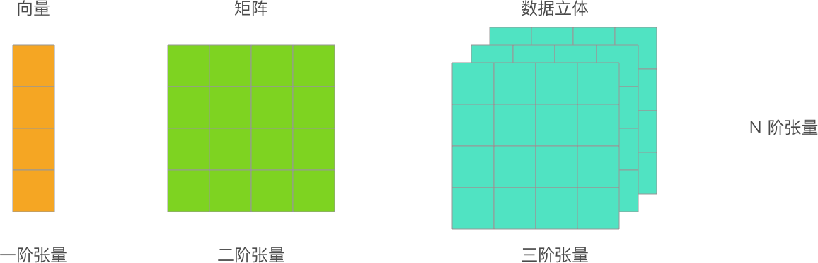
https://cdn.aibydoing.com/aibydoing/images/document-uid214893labid6102timestamp1532052623486.png

So, tensors are not some esoteric concept. Speaking loosely, a tensor is an N-dimensional array. Vectors and matrices mentioned earlier are also tensors. Most deep learning frameworks you will learn about later will use the concept of tensors, and the advantage of doing so is to unify the definition of data. In NumPy, data is defined using Ndarray multi-dimensional arrays, and in TensorFlow, data is represented using tensors.

50.4.1. Tensor Types#

In TensorFlow, every tensor has three basic attributes: data, data type, and shape. And according to different uses, tensors are divided into two types, namely:

tf.Variable: A variable Tensor that requires an initial value and is commonly used to define mutable parameters, such as the weights of a neural network.
tf.constant: A constant Tensor that requires an initial value and defines an unchanging tensor.

We can create tensors of variable and constant types by passing in arrays:

                            import tensorflow as tf

v = tf.Variable([[1, 2], [3, 4]])  # 形状为 (2, 2) 的二维变量
v

                            <tf.Variable 'Variable:0' shape=(2, 2) dtype=int32, numpy=
array([[1, 2],
       [3, 4]], dtype=int32)>

                          

                            c = tf.constant([[1, 2], [3, 4]])  # 形状为 (2, 2) 的二维常量
c

                            <tf.Tensor: shape=(2, 2), dtype=int32, numpy=
array([[1, 2],
       [3, 4]], dtype=int32)>

                          

Look closely and you will find that the output contains three attributes of the tensor, namely the shape shape, the data type dtype, and the corresponding NumPy array.

We can directly output the NumPy array of a tensor through .numpy().

                            c.numpy()

                          

                            array([[1, 2],
       [3, 4]], dtype=int32)

50.4.2. Common Tensors#

Above, we have introduced constant tensors. Here are several commonly used methods for creating constant tensors that are often used:

tf.zeros: Create a constant Tensor of all zeros with the specified shape.
tf.zeros_like: Create a constant Tensor of all zeros with a shape based on a reference.
tf.ones: Create a constant Tensor of all ones with the specified shape.
tf.ones_like: Create a constant Tensor of all ones with a shape based on a reference.
tf.fill: Create a constant Tensor of a specified shape filled with a scalar value.

                            tf.zeros([3, 3])  # 3x3 全为 0 的常量 Tensor

                          

                            <tf.Tensor: shape=(3, 3), dtype=float32, numpy=
array([[0., 0., 0.],
       [0., 0., 0.],
       [0., 0., 0.]], dtype=float32)>

                          

                            tf.ones_like(c)  # 与 c 形状一致全为 1 的常量 Tensor

                          

                            <tf.Tensor: shape=(2, 2), dtype=int32, numpy=
array([[1, 1],
       [1, 1]], dtype=int32)>

                          

                            tf.fill([2, 3], 6)  # 2x3 全为 6 的常量 Tensor

                          

                            <tf.Tensor: shape=(2, 3), dtype=int32, numpy=
array([[6, 6, 6],
       [6, 6, 6]], dtype=int32)>

                          

In addition, we can also create some sequences, such as:

tf.linspace: Create an equally-spaced sequence.
tf.range: Create a sequence of numbers.

                            tf.linspace(1.0, 10.0, 5)  # 从 1 到 10，共 5 个等间隔数

                          

                            <tf.Tensor: shape=(5,), dtype=float32, numpy=array([ 1.  ,  3.25,  5.5 ,  7.75, 10.  ], dtype=float32)>

                          

                            tf.range(start=1, limit=10, delta=2)  # 从 1 到 10 间隔为 2

                          

<tf.Tensor: shape=(5,), dtype=int32, numpy=array([1, 3, 5, 7, 9], dtype=int32)>

If you are familiar with NumPy, you will find that this is similar to the methods of creating various multi-dimensional arrays in NumPy. After understanding tensors, we can continue to learn the tensor operation mechanism in TensorFlow.

Note

It is impossible to memorize all the tensor methods in TensorFlow at once. You can only become familiar with them through continuous use. Most of the time, we have a need first. For example, you need to generate equally-spaced numbers. At this time, you can then search the official documentation to see if there is a corresponding ready-made function available. The methods provided by TensorFlow basically meet various common needs.

50.5. Eager Execution#

One of the biggest changes brought by TensorFlow 2 is changing the Graph Execution (graph and session mechanism) in 1.x to Eager Execution (dynamic graph mechanism). In the 1.x version, the low-level TensorFlow API first needed to define a data flow graph and then create a TensorFlow session, which is completely abandoned in 2.0. Eager Execution in TensorFlow 2 is an imperative programming environment that evaluates operations immediately without building a graph.

Therefore, the tensor operation process in TensorFlow can be as intuitive and natural as in NumPy. Next, let’s take the simplest addition operation as an example:

                          c + c  # 加法计算

                        

                          <tf.Tensor: shape=(2, 2), dtype=int32, numpy=
array([[2, 4],
       [6, 8]], dtype=int32)>

                        

If you have worked with TensorFlow 1.x, you should know that the process of an addition operation is quite complex. We need to initialize global variables → create a session → execute the calculation, and finally we can print out the result of the tensor operation.

# TensorFlow 1.x implementation code for the above addition operation
init_op = tf.global_variables_initializer()  # Initialize global variables
with tf.Session() as sess:  # Start a session
    sess.run(init_op)
    print(sess.run(c + c))  # Execute the calculation

The benefits brought by Eager Execution are obvious. It further lowers the entry threshold of TensorFlow. The previous Graph Execution mode actually made many beginners feel frustrated when getting started because it completely didn’t conform to normal thinking habits.

The mathematical calculations provided in TensorFlow, including methods for linear algebra calculations, are also应有尽有 and very rich. Below, we list an example.

                          a = tf.constant([1.0, 2.0, 3.0, 4.0, 5.0, 6.0], shape=[2, 3])
b = tf.constant([7.0, 8.0, 9.0, 10.0, 11.0, 12.0], shape=[3, 2])

c = tf.linalg.matmul(a, b)  # 矩阵乘法
c

                          <tf.Tensor: shape=(2, 2), dtype=float32, numpy=
array([[ 58.,  64.],
       [139., 154.]], dtype=float32)>

                        

                          tf.linalg.matrix_transpose(c)  # 转置矩阵

                        

                          <tf.Tensor: shape=(2, 2), dtype=float32, numpy=
array([[ 58., 139.],
       [ 64., 154.]], dtype=float32)>

                        

You should be able to feel that corresponding methods for these common APIs can be found in NumPy, which is why the course requires you to be familiar with NumPy in advance. Due to the close integration of TensorFlow and NumPy, even if a calculation function available in NumPy is not provided in TensorFlow, you can first use NumPy to complete the calculation and then convert it to a TensorFlow tensor representation. Since there are so many functions, generally speaking, except for those you often use, you will consult the official documentation when you need a certain operation.

50.6. Automatic Differentiation#

In mathematics, differentiation is a linear description of the local rate of change of a function. Although differentiation and derivative are two different concepts. However, for a univariate function, differentiability and derivability are completely equivalent. Previously, we have been familiar with the process of building a neural network, and you should understand the importance of gradients. And the differentiation process for complex functions is extremely troublesome. To improve application efficiency, most deep learning frameworks have an automatic differentiation mechanism.

Next, we demonstrate an automatic differentiation process. Suppose a mathematical derivative calculation process is as follows:

\[ loss = w^2 \rightarrow \frac {\partial loss}{\partial w} = 2w \]

So, when \(w\) equals 1, the calculation result is 2.

In TensorFlow, you can use tf.GradientTape to track the entire operation process so as to calculate gradients when necessary.

                          w = tf.Variable([1.0])  # 新建张量

with tf.GradientTape() as tape:  # 追踪梯度
    loss = w * w  # 计算过程

tape.gradient(loss, w)  # 计算梯度

<tf.Tensor: shape=(1,), dtype=float32, numpy=array([2.], dtype=float32)>

tf.GradientTape records gradient information in the computational graph like a tape, and then the .gradient can be used to backtrack and calculate any gradient, which is very important for updating parameters when building neural networks using TensorFlow’s low-level API.

50.7. Common Modules#

Above, we have learned the core knowledge of TensorFlow. Next, we will give a brief introduction to the functions of common modules in the TensorFlow API. The use of the framework is actually about flexibly applying various encapsulated classes and functions. Since the number of TensorFlow APIs is too large and the iteration is too fast, everyone should develop the habit of consulting the official documentation at any time.

tf.: Contains common functions and classes such as tensor definitions and transformations.
tf.data: Input data processing module, providing classes like tf.data.Dataset to encapsulate input data and specify batch sizes, etc.
tf.image: Image processing module, providing classes for image cropping, transformation, encoding, decoding, etc.
tf.keras: The high-level API of the original Keras framework. It contains high-level neural network layers from the original tf.layers.
tf.linalg: Linear algebra module, providing a large number of linear algebra calculation methods and classes.
tf.losses: Loss function module, used to conveniently define loss functions for neural networks.
tf.math: Mathematical calculation module, providing a large number of mathematical calculation functions.
tf.saved_model: Model saving module, which can be used for model saving and restoration.
tf.train: Provides components for training, such as optimizers, learning rate decay strategies, etc.
tf.nn: Provides low-level functions for building neural networks to help implement various functional layers of deep neural networks.
tf.estimator: High-level API, providing pre-created Estimators or custom components.

When building a deep neural network, TensorFlow can be said to provide all the components you want, from tensors of different shapes, activation functions, neural network layers, to optimizers, datasets, etc. Since TensorFlow contains too many interfaces, it becomes impractical to practice each one separately. Therefore, we will introduce them in detail when we use the corresponding functions later.

Note

When learning, you can quickly browse through the methods included in each main module of TensorFlow via the hyperlinks above. There’s no need to memorize them; just leave a basic impression, which will be very helpful for you to understand the overall picture of TensorFlow.

50.8. Summary#

TensorFlow is a very powerful framework, and many people who have used it for a long time still dare not claim to have learned it well. When learning such a large and complex framework, the right approach is not to try to take a huge bite all at once, but to take it one bite at a time. In this section of the experiment, we learned about the working mechanism of TensorFlow’s Eager Execution, studied tensors and the method of automatic differentiation, and also sorted out the common modules and functions in TensorFlow.