Pro Membership

Pro Membership is a membership plan created by the author to maintain and update this tutorial. You can get more benefits and services, click to view details.

93. Basic Pandas Data Processing#

93.1. Introduction#

Pandas is a very well-known open-source data processing library through which we can perform a series of operations on datasets, such as quickly reading, transforming, filtering, and analyzing them. In addition, Pandas has powerful capabilities for handling missing data and data pivoting, making it an essential tool in data preprocessing.

93.2. Key Points#

Data types
Data reading
Data selection
Data deletion
Data filling

https://cdn.aibydoing.com/aibydoing/images/uid214893-20200506-1588754125824.svg

Pandas is a very well-known open-source data processing library. It is developed based on NumPy and is designed to solve data analysis tasks in the Scipy ecosystem. Pandas incorporates a large number of libraries and some standard data models, providing the functions and methods required to efficiently operate on large datasets.

The unique data structures are the advantages and core of Pandas. Simply put, we can convert data in any format into Pandas data types and use a series of methods provided by Pandas for conversion and operation to finally obtain the results we expect.

Therefore, we first need to understand and be familiar with the data types supported by Pandas.

93.3. Data Types#

The main data types in Pandas are as follows: Series (one-dimensional array), DataFrame (two-dimensional array), Panel (three-dimensional array), Panel4D (four-dimensional array), and PanelND (more-dimensional arrays). Among them, Series and DataFrame are the most widely used, accounting for more than 90% of the usage frequency.

93.4. Series#

Series is the most basic one-dimensional array form in Pandas. It can store data of types such as integers, floating-point numbers, and strings. The basic structure of Series is as follows:

                      pandas.Series(data=None, index=None)

                    

Among them, data can be a dictionary, or an ndarray object in NumPy, etc. index is the data index. Indexing is a major feature in Pandas data structures, and its main function is to help us locate data more quickly.

Next, we create an example Series based on a Python dictionary.

                          %matplotlib inline
import pandas as pd

s = pd.Series({'a': 10, 'b': 20, 'c': 30})
s

As shown above, the data values of this Series are 10, 20, 30, the index is a, b, c, and the type of the data values is recognized as int64 by default. You can use type to confirm the type of s.

                          type(s)

                        

Since Pandas is developed based on NumPy. Then the data type ndarray of multi-dimensional arrays in NumPy can naturally be converted into data in Pandas. And Series can be converted based on one-dimensional data in NumPy.

                          import numpy as np

s = pd.Series(np.random.randn(5))
s

As shown above, we presented a one-dimensional random array generated by NumPy. The resulting Series has an index that by default starts from 0, and the numerical type is float64.

93.5. DataFrame#

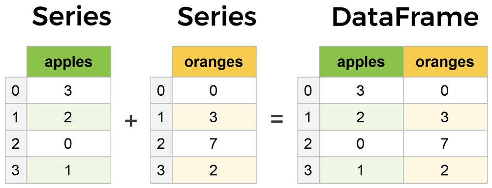
DataFrame is the most common, important, and frequently used data structure in Pandas. A DataFrame is similar to a normal spreadsheet or SQL table structure. You can think of a DataFrame as an extended type of Series, as if it were composed of multiple Series combined. The intuitive difference between it and Series is that the data has not only row indices but also column indices.

Source

The basic structure of a DataFrame is as follows:

                      pandas.DataFrame(data=None, index=None, columns=None)

                    

Different from Series, it adds a columns column index. A DataFrame can be constructed from the following multiple types of data:

One-dimensional arrays, lists, dictionaries, or Series dictionaries.
Two-dimensional or structured numpy.ndarray.
A Series or another DataFrame.

For example, we first use a dictionary consisting of Series to construct a DataFrame.

                          df = pd.DataFrame({'one': pd.Series([1, 2, 3]),
                   'two': pd.Series([4, 5, 6])})
df

                        

When no index is specified, the index of the DataFrame also starts from 0. We can also directly generate a DataFrame through a dictionary composed of a list.

                          df = pd.DataFrame({'one': [1, 2, 3],
                   'two': [4, 5, 6]})
df

                        

Or, conversely, generate a DataFrame from a list with a dictionary.

                          df = pd.DataFrame([{'one': 1, 'two': 4},
                   {'one': 2, 'two': 5},
                   {'one': 3, 'two': 6}])
df

                        

Multidimensional arrays in NumPy are very commonly used, and a DataFrame can also be constructed based on two-dimensional numerical values.

                          pd.DataFrame(np.random.randint(5, size=(2, 4)))

                        

At this point, you should already be clear about the commonly used Series and DataFrame data types in Pandas. A Series can actually be roughly regarded as a DataFrame with only one column of data. Of course, this statement is not rigorous, and the core difference between the two is still that a Series does not have a column index. You can observe the Series and DataFrame generated from a one-dimensional random NumPy array as shown below.

                          pd.Series(np.random.randint(5, size=(5,)))

                        

                          pd.DataFrame(np.random.randint(5, size=(5,)))

                        

We will no longer introduce data types such as Panel in Pandas. Firstly, these data types are rarely used. Secondly, even if you use them, you can apply the skills learned from DataFrame and others for migration. The principle remains the same despite all changes.

93.6. Data Reading#

If we want to analyze data using Pandas, we first need to read the data. In most cases, the data comes from external data files or databases. Pandas provides a series of methods to read external data, which is very comprehensive. Below, we will introduce it using the most commonly used CSV data file as an example.

The method to read a CSV file is pandas.read_csv(), and you can directly pass in a relative path or a network URL.

                          df = pd.read_csv("https://cdn.aibydoing.com/aibydoing/files/los_census.csv")
df

Since a CSV is stored as a two-dimensional table, Pandas will automatically read it as a DataFrame type.

Now you should understand that the DataFrame is the core of Pandas. All data, whether read externally or generated by ourselves, we need to first convert it into the DataFrame or Series data types of Pandas. In fact, in most cases, all of this is already designed and no additional conversion work needs to be performed.

The methods starting with the prefix pd.read_ can also read various data files and support connecting to databases. Here, we will not elaborate one by one. You can read the corresponding section of the official documentation to familiarize yourself with these methods and understand the parameters included in these methods.

You may have another question: Why do we need to convert data into Series or DataFrame structures?

In fact, I can answer this question right now. Because all the methods of Pandas for data manipulation are designed based on the data structures supported by Pandas. That is to say, only Series or DataFrame can be processed using the methods and functions provided by Pandas. Therefore, before learning the real data processing methods, we need to convert the data into Series or DataFrame types.

93.7. Basic Operations#

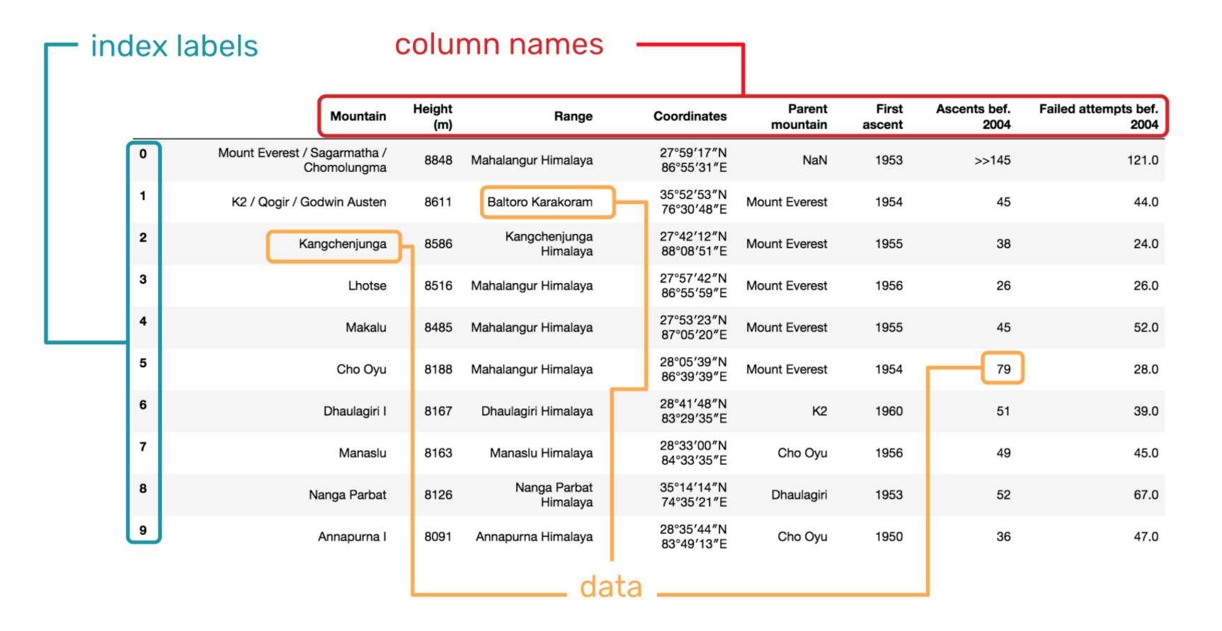
From the above content, we already know that a DataFrame structure generally consists of three parts, namely column names, index, and data.

Source

Next, we will learn the basic operations on DataFrame. In this chapter, we will not deliberately emphasize Series because most of the methods and techniques you learn on DataFrame are applicable to processing Series. They share the same origin.

Above, we have read an external data, which is the census data of Los Angeles. Sometimes, the files we read are very large. If we output and preview all of these files, it is neither beautiful nor time-efficient. Fortunately, Pandas provides the head() and tail() methods, which can help us preview only a small piece of data.

                          df.head()  # 默认显示前 5 条

                        

                          df.tail(7)  # 指定显示后 7 条

                        

Pandas also provides statistical and descriptive methods to help you understand the dataset from a macroscopic perspective. describe() is equivalent to providing an overview of the dataset and will output the count, maximum value, minimum value, etc. of each column in the dataset.

                          df.describe()

                        

Pandas is developed based on NumPy, so at any time you can convert a DataFrame to a NumPy array via .values.

                          df.values

                        

This also means that you can operate on the same data using the APIs provided by both Pandas and NumPy and freely convert between the two. This is a very flexible tool ecosystem.

In addition to .values, the common attributes supported by DataFrame can be viewed through the corresponding section of the official documentation. Among them, the commonly used ones are:

                          df.index  # 查看索引

                        

                          df.columns  # 查看列名

                        

                          df.shape  # 查看形状

                        

93.8. Data Selection#

During the data preprocessing process, we often split the dataset and only retain certain rows, columns, or data blocks that we need, and output them to the next process. This is what we call data selection, or data indexing.

Since there are indexes and labels in the data structures of Pandas, we can complete data selection through multi-axis indexing.

93.9. Selection Based on Index Numbers#

When we create a new DataFrame, if we don’t specify the row index or the column corresponding labels ourselves, then Pandas will default to using numbers starting from 0 as the row index and the first row of the dataset as the column corresponding labels. In fact, there are also numerical indexes for the “columns” here, which also default to starting from 0, but are not displayed.

Therefore, we can first select the dataset based on numerical indexes. Here we use the .iloc method in Pandas. The types that this method can accept are:

Integers. For example: 5
Lists or arrays composed of integers. For example: [1, 2, 3]
Boolean arrays.
Functions or arguments that can return index values.

Next, we use the example data above for demonstration.

First, we can select the first 3 rows of data. This is very similar to slicing in Python or NumPy.

                          df.iloc[:3]

                        

We can also select a specific row.

                          df.iloc[5]

                        

So, to select multiple rows, is it like df.iloc[1, 3, 5]?

The answer is incorrect. In df.iloc[], the [[rows], [columns]] can accept the positions of rows and columns simultaneously. If you directly type df.iloc[1, 3, 5], it will result in an error.

So, it’s very simple. If you want to select rows 2, 4, and 6, you can do it like this.

                          df.iloc[[1, 3, 5]]

                        

After learning how to select rows, you should be able to figure out how to select columns. For example, if we want to select columns 2 - 4.

                          df.iloc[:, 1:4]

                        

Here, to select columns 2 - 4, what is entered is 1:4. This is very similar to the slicing operation in Python or NumPy. Since we can locate rows and columns, then by just combining them, we can select any data in the dataset.

93.10. Selection Based on Label Names#

In addition to selecting based on numerical indices, you can also directly select based on the names corresponding to the labels. The method used here is very similar to iloc above, but without the i, which is [df.loc[]](https://pandas.pydata.org/pandas-docs/stable/reference/api/pandas.DataFrame.loc.html#pandas.DataFrame.loc).

The types that df.loc[] can accept are:

A single label. For example: 2 or 'a', where 2 refers to the label rather than the index position.
A list or array of labels. For example: ['A', 'B', 'C'].
A slice object. For example: 'A':'E', note the difference from the slicing above, both the start and end are included.
A boolean array.
A function or a callable that returns labels.

Next, let’s demonstrate the usage of df.loc[]. First, select the first 3 rows:

                          df.loc[0:2]

                        

Then select rows 1, 3, and 5:

                          df.loc[[0, 2, 4]]

                        

Then, select columns 2 - 4:

                          df.loc[:, 'Total Population':'Total Males']

                        

Finally, select rows 1, 3 and the columns after Median Age:

                          df.loc[[0, 2], 'Median Age':]

                        

93.11. Data Deletion#

Although we can obtain the data we need from a complete dataset through data selection methods, sometimes it is simpler and more straightforward to directly delete the unnecessary data. In Pandas, methods starting with .drop are related to data deletion.

DataFrame.drop can directly remove the specified columns and rows from the dataset. Generally, when using it, we specify the labels label parameter, and then use axis to specify whether to delete by column or by row. Of course, you can also delete data through index parameters. For specific details, please refer to the official documentation.

                          df.drop(labels=['Median Age', 'Total Males'], axis=1)

                        

DataFrame.drop_duplicates is usually used for data deduplication, that is, removing duplicate values from the dataset. The usage method is very simple. By default, it will delete duplicate rows based on all columns. You can also use subset to specify the duplicates on specific columns to be deleted. To delete duplicates and keep the last occurrence, use keep=‘last’.

                          df.drop_duplicates()

                        

In addition, another method for data deletion, DataFrame.dropna, is also very commonly used. Its main purpose is to delete missing values, that is, the missing data columns or rows in the dataset.

                          df.dropna()

                        

For the three commonly used data deletion methods mentioned above, you must read the official documentation through the provided links. There are not many things to note about these commonly used methods. Just understand their usage through the documentation. Therefore, we will not introduce them in a complicated way.

93.12. Data Filling#

Since data deletion has been mentioned, conversely, we may encounter the situation of data filling. For a given dataset, we generally don’t fill data randomly, but rather fill in the missing values more often.

In a real production environment, the data files we need to process are often not as ideal as we imagine. Among them, the situation of missing values is very likely to be encountered. Missing values mainly refer to the phenomenon of data loss, that is, a certain piece of data in the dataset does not exist. In addition, data that exists but is obviously incorrect is also classified as missing values. For example, in a time series dataset, if the time flow of a certain segment of data suddenly gets disrupted, then this small piece of data is meaningless and can be classified as a missing value.

93.13. Detecting Missing Values#

To more conveniently detect missing values, Pandas uses NaN to mark the missing values of different types of data. Here, NaN stands for Not a Number, and it is just used as a marker. An exception is that in a time series, the loss of a timestamp is marked with NaT.

In Pandas, two main methods are used to detect missing values, namely: isna() and notna(). As the names imply, they mean “is a missing value” and “is not a missing value” respectively. By default, they return boolean values for judgment.

Next, we artificially generate a set of sample data containing missing values.

                          df = pd.DataFrame(np.random.rand(9, 5), columns=list('ABCDE'))
# 插入 T 列，并打上时间戳
df.insert(value=pd.Timestamp('2017-10-1'), loc=0, column='Time')
# 将 1, 3, 5 列的 2，4，6，8 行置为缺失值
df.iloc[[1, 3, 5, 7], [0, 2, 4]] = np.nan
# 将 2, 4, 6 列的 3，5，7，9 行置为缺失值
df.iloc[[2, 4, 6, 8], [1, 3, 5]] = np.nan
df

                        

Then, you can determine the missing values in the dataset by using either isna() or notna().

                          df.isna()

                        

The generation and detection of default values have been introduced above. In fact, when dealing with missing values, there are generally two operations: filling and removing. Both filling and clearing are two extremes. If you feel it is necessary to retain the columns or rows where the missing values are located, then you need to fill in the missing values. If there is no need to retain them, you can choose to remove the missing values.

Among them, the method dropna() for removing missing values has been introduced above. Now let’s take a look at the method fillna() for filling missing values.

First, we can replace NaN with the same scalar value, such as 0.

                          df.fillna(0)

                        

In addition to directly filling the values, we can also fill the corresponding missing values with the values before or after the missing values through parameters. For example, filling with the value before the missing value:

                          df.fillna(method='pad')

                        

Or the value after it:

                          df.fillna(method='bfill')

                        

The last row still has missing values because there is no subsequent value for it.

In the above example, our missing values are present at intervals. So, what if there are consecutive missing values? Give it a try. First, we also set the 3rd and 5th rows of the 2nd, 4th, and 6th columns of the dataset as missing values.

                          df.iloc[[3, 5], [1, 3, 5]] = np.nan

                        

Then perform forward filling:

                          df.fillna(method='pad')

                        

As can be seen, consecutive missing values are also filled according to the previous values and are completely filled. Here, we can set the limit number of consecutive fills through the limit= parameter.

                          df.fillna(method='pad', limit=1)  # 最多填充一项

                        

In addition to the above filling methods, we can also fill specific columns or rows by using the built-in methods of Pandas to calculate the average value. For example:

                          df.fillna(df.mean()['C':'E'])

                        

Fill columns C to E with the average value.

93.14. Interpolation Filling#

Interpolation is a method in numerical analysis. Briefly speaking, it is to solve the value of unknown data by means of a function (linear or non-linear) based on known data. Interpolation is very common in the field of data, and its advantage is that it can try to restore the original appearance of the data as much as possible.

We can complete linear interpolation through the interpolate() method (https://pandas.pydata.org/pandas-docs/stable/reference/api/pandas.DataFrame.interpolate.html#pandas.DataFrame.interpolate). Of course, some other interpolation algorithms can be learned by reading the official documentation.

                          # 生成一个 DataFrame
df = pd.DataFrame({'A': [1.1, 2.2, np.nan, 4.5, 5.7, 6.9],
                   'B': [.21, np.nan, np.nan, 3.1, 11.7, 13.2]})
df

                        

For the missing values that exist above, it is not very effective to fill them with the previous and next values or the average value, as this may not reflect the trend well. In this case, interpolation is the best option. Let’s try using the default linear interpolation.

                          df_interpolate = df.interpolate()
df_interpolate

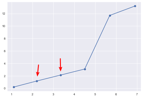
The following figure shows the data after interpolation, and it is obvious that the interpolation result conforms to the changing trend of the data. If filled according to the order of the previous and subsequent data, this cannot be achieved.

For the interpolation algorithms supported by interpolate() (https://pandas.pydata.org/pandas-docs/stable/reference/api/pandas.DataFrame.interpolate.html#pandas.DataFrame.interpolate), that is, method=. The following are several suggestions for selection:

If the growth rate of your data is increasing, you can choose method='quadratic' for quadratic interpolation.
If the dataset呈现出累计分布的样子, it is recommended to choose method='pchip'.
If you need to fill in missing values and aim to smooth the plot, it is recommended to choose method='akima'.

Of course, for the last-mentioned method='akima', the Scipy library needs to be installed in your environment. In addition, method='barycentric' and method='pchip' also require Scipy to be used.

93.15. Data Visualization#

NumPy, Pandas, and Matplotlib form a complete data analysis ecosystem, so the compatibility of the three tools is very good, and they even share a large number of interfaces. When our data is presented in the DataFrame format, we can directly use the DataFrame.plot method provided by Pandas (https://pandas.pydata.org/pandas-docs/stable/reference/frame.html#plotting) to call the Matplotlib interface to draw common graphs.

For example, we use the interpolated data df_interpolate above to draw a line chart.

                          df_interpolate.plot()

                        

Other styles of graphs are also very simple. Just specify the kind= parameter.

                          df_interpolate.plot(kind='bar')

                        

For more graph styles and parameters, read the detailed instructions in the official documentation. Although Pandas plotting cannot achieve the flexibility of Matplotlib, it is simple and easy to use, suitable for the quick presentation and preview of data.

93.16. Other Usages#

Since Pandas contains so much content, it is difficult to have a comprehensive understanding through a single experiment or course, other than reading the complete official documentation. Of course, the purpose of this chapter is to familiarize you with the commonly used basic methods of Pandas. At least you generally know what Pandas is and what it can do.

In addition to some of the methods and techniques mentioned above, what Pandas commonly uses actually also includes:

Data Calculation, such as: DataFrame.add, etc.
Data Aggregation, such as: DataFrame.groupby, etc.
Statistical Analysis, such as: DataFrame.abs, etc.
Time Series, such as: DataFrame.shift, etc.

93.17. Summary#

In this experiment, we mainly introduced the data structures of Pandas. You need to have a deep understanding of Series and DataFrame in order to have a more profound understanding of data preprocessing using Pandas later. In addition, we learned the methods and techniques of data reading, data selection, data deletion, and data filling in Pandas. We hope that everyone can further deepen their understanding in combination with the official documentation in the future.

○ Sharethis article link to your social media, blog, forum, etc. More external links will increase the search engine ranking of this site.

If you find this content helpful, you can buy me a coffee

92. NumPy Numerical Computing Basics

94. Matplotlib 2D Image Plotting Methods