
19. Support Vector Machine for Portrait Classification#
19.1. Introduction#
Support Vector Machine is a very excellent algorithm. In this challenge, we will use the Support Vector Machine method provided by scikit-learn to complete the face image classification task.
19.2. Key Points#
Image data preprocessing
Support Vector Machine classification
First, we download the face dataset through
fetch_lfw_people
provided by scikit-learn. The dataset was originally from
the
Labeled Faces in the Wild
project.
from sklearn.datasets import fetch_lfw_people

# 加载数据集
faces = fetch_lfw_people(min_faces_per_person=60)
faces.target_names, faces.images.shape
(array(['Ariel Sharon', 'Colin Powell', 'Donald Rumsfeld', 'George W Bush',
        'Gerhard Schroeder', 'Hugo Chavez', 'Junichiro Koizumi',
        'Tony Blair'], dtype='<U17'),
 (1348, 62, 47))
As can be seen, we only used the portrait data of 8 famous
people, with a total of 1,348 samples. Among them, the size
of each portrait photo is 62 * 47 pixels. The summary of the
faces
attribute is as follows:
Attribute |
Description |
|---|---|
|
|
62x47 matrix recording pixel values in face images |
|
|
Converts the 62x47 matrix corresponding to
|
|
|
Names of 8 portraits |
|
|
Sequential numbers of 8 portraits |
Next, we first use Matplotlib plotting to preview this data.
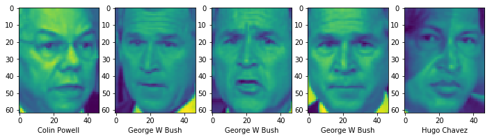
Exercise 19.1
Challenge: Preview the first 5 portrait images in the dataset and present them as a subplot with 1 row and 5 columns.
Requirement: Display the name of the portrait corresponding to each image on the horizontal axis of each image.
from matplotlib import pyplot as plt

%matplotlib inline

## 代码开始 ### (≈4 行代码)

## 代码结束 ###
Solution to Exercise 19.1
from matplotlib import pyplot as plt
%matplotlib inline

### Code start ### (≈4 lines of code)
fig, axes = plt.subplots(1, 5, figsize=(12, 6))
for i, image in enumerate(faces.images[:5]):
    axes[i].imshow(image)
    axes[i].set_xlabel(faces.target_names[faces.target[i]])
### Code end ###
Expected output
Since the images themselves are 2D arrays, they need to be
processed before being used to train the model. Therefore,
below we use the
faces.data
data, which has flattened the 2D array corresponding to each
portrait into a 1D array.
faces.data.shape
It can be seen that the shape of
faces.data
is
\((1348, 2914)\), which means there are 1348 samples, and each sample
corresponds to 2914 features. These 2914 features are the
vectors after flattening the portrait images of
\(62*47 = 2914\).
Next, as usual, it is necessary to split the dataset into a training set and a test set. However, it should be noted here that since there are only 1348 samples and each sample corresponds to 2914 features. In the process of machine learning modeling, we should avoid the situation where the number of features is much larger than the number of samples, as the models trained in this way generally perform very poorly.
Therefore, here we need to perform “dimensionality reduction” on the data features, which actually means reducing the number of data features. Here we use the PCA dimensionality reduction method, which will be introduced in detail in subsequent experiments and will not be explained here.
from sklearn.decomposition import PCA

# 直接运行,将数据特征缩减为 150 个
pca = PCA(n_components=150, whiten=True, random_state=42)
pca_data = pca.fit_transform(faces.data)
pca_data.shape
It can be seen that the shape of the data has changed from the previous \((1348, 2914)\) to \((1348, 150)\).
Next, the training set and the test set can be split based on the dimension-reduced data.
Exercise 19.2
Challenge: Use
train_test_split()
to split the dataset into two parts: 80% (training set)
and 20% (test set).
Specification: The training set features, test set
features, training set target, and test set target are
X_train,
X_test,
y_train, and
y_test
respectively, and the random seed is set to 42.
from sklearn.model_selection import train_test_split

## 代码开始 ### (≈1 行代码)

## 代码结束 ###

X_train.shape, X_test.shape, y_train.shape, y_test.shape
Solution to Exercise 19.2
from sklearn.model_selection import train_test_split

### Code starts ### (≈1 line of code)
X_train, X_test, y_train, y_test = train_test_split(
    pca_data, faces.target, test_size=0.2, random_state=42)
### Code ends ###

X_train.shape, X_test.shape, y_train.shape, y_test.shape
Expected output
((1078, 150), (270, 150), (1078,), (270,))
Next, we use the SVM algorithm to build a model and train and test the model using the data split above.
Exercise 19.3
Challenge: Use the support vector machine classification method provided by scikit-learn to complete the modeling and obtain the accuracy result of the model on the test set.
Requirement: The parameters of the support vector
machine classifier are
C
                          =
                          10
and
gamma
                          =
                          0.001
, and the rest are default parameters.
## 代码开始 ### (≈4 行代码)
model = None
## 代码结束 ###
Solution to Exercise 19.3
### Code starts ### (≈4 lines of code)
from sklearn.svm import SVC

model = SVC(C=10, gamma=0.001)
model.fit(X_train, y_train)
model.score(X_test, y_test)
### Code ends ###
Expected output
The final accuracy > 0.8 is sufficient.