
10. Comprehensive Application Exercises of Regression Methods#
10.1. Introduction#
This challenge will combine the relevant regression analysis methods learned previously to complete a multiple regression analysis task. At the same time, we will review the implementation and application of different methods by combining libraries such as NumPy, scikit-learn, SciPy, and statsmodels.
10.2. Key Points#
Simple linear regression
Multiple linear regression
Hypothesis testing
The challenge uses the
Advertising
example dataset provided in the book
An Introduction to Statistical Learning for
practice. This book is a classic in statistical learning. If
you are interested, you can
download and read it for free
from the author’s website.
First, we load and preview the dataset.
# 下载数据集
!wget -nc https://cdn.aibydoing.com/aibydoing/files/advertising.csv
import pandas as pd

data = pd.read_csv("advertising.csv", index_col=0,)
data.head()
| tv | radio | newspaper | sales | |
|---|---|---|---|---|
| 1 | 230.1 | 37.8 | 69.2 | 22.1 |
| 2 | 44.5 | 39.3 | 45.1 | 10.4 |
| 3 | 17.2 | 45.9 | 69.3 | 9.3 |
| 4 | 151.5 | 41.3 | 58.5 | 18.5 |
| 5 | 180.8 | 10.8 | 58.4 | 12.9 |
The dataset contains 4 columns and 200 rows in total. Each sample represents the advertising expenses required for a supermarket to sell a corresponding unit of goods. Taking the first row as an example, it means that for the supermarket to sell an average of 22.1 units of goods, the advertising expenses for TV, radio, and newspaper are: \(230.1, \)37.8, and $69.2 respectively.
Therefore, in this challenge, the first 3 columns are regarded as features and the last column as the target value.
Exercise 10.1
Challenge: Use the ordinary least squares method provided by SciPy to calculate the fitting parameters of the univariate linear regression model between the three features and the target respectively.
Requirement: The
scipy.optimize.leastsq
function should be used to complete the calculation, and
the function result should be directly output without
processing.
import numpy as np
from scipy.optimize import leastsq

## 代码开始 ### (≈ 10 行代码)
params_tv = None
params_radio = None
params_newspaper = None
## 代码结束 ###

params_tv[0], params_radio[0], params_newspaper[0]
Solution to Exercise 10.1
import numpy as np
from scipy.optimize import leastsq

### Code start ### (≈ 10 lines of code)
p_init = np.random.randn(2)

def func(p, x):
    w0, w1 = p
    f = w0 + w1*x
    return f

def err_func(p, x, y):
    ret = func(p, x) - y
    return ret

params_tv = leastsq(err_func, p_init, args=(data.tv, data.sales))
params_radio = leastsq(err_func, p_init, args=(data.radio, data.sales))
params_newspaper = leastsq(err_func, p_init, args=(data.newspaper, data.sales))
### Code end ###

params_tv[0], params_radio[0], params_newspaper[0]
Expected output
((array([7.03259354, 0.04753664]),
 (array([9.31163807, 0.20249578]),
 (array([12.35140711, 0.0546931]))
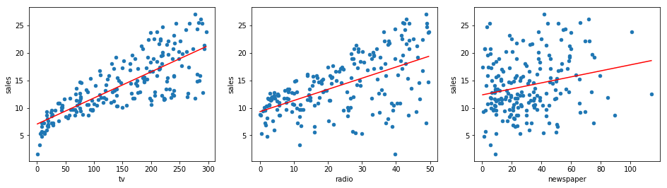
Next, based on the results obtained by the least squares method, we plot the fitted line onto the original scatter plot of the distribution.
Exercise 10.2
Challenge: Plot the scatter plots between the three features and the target respectively in a horizontal subplot manner, and add the linear fitting lines.
Requirement: The linear fitting lines start from the minimum abscissa value in the scatter plot, end at the maximum abscissa value, and are shown in red.
from matplotlib import pyplot as plt

%matplotlib inline

## 代码开始 ### (≈ 10 行代码)


## 代码结束 ###
Solution to Exercise 10.2
from matplotlib import pyplot as plt
%matplotlib inline

### Code start ### (≈ 10 lines of code)
fig, axes = plt.subplots(1, 3, figsize=(16, 4))

data.plot(kind='scatter', x='tv', y='sales', ax=axes[0])
data.plot(kind='scatter', x='radio', y='sales', ax=axes[1])
data.plot(kind='scatter', x='newspaper', y='sales', ax=axes[2])

x_tv = np.array([data.tv.min(), data.tv.max()])
axes[0].plot(x_tv, params_tv[0][1]*x_tv + params_tv[0][0], 'r')

x_radio = np.array([data.radio.min(), data.radio.max()])
axes[1].plot(x_radio, params_radio[0][1]*x_radio + params_radio[0][0], 'r')

x_newspaper = np.array([data.newspaper.min(), data.newspaper.max()])
axes[2].plot(x_newspaper, params_newspaper[0][1] *
             x_newspaper + params_newspaper[0][0], 'r')
### Code end ###
Expected output
Next, we try to build a multiple linear regression model that includes all features.
Exercise 10.3
Challenge: Use the linear regression method provided by scikit-learn to build a multiple linear regression model consisting of 3 features and a target.
Requirement: Only the
sklearn.linear_model.LinearRegression
class provided by scikit-learn can be used.
from sklearn.linear_model import LinearRegression

## 代码开始 ### (≈ 4 行代码)
model = None
## 代码结束 ###

model.coef_, model.intercept_  # 返回模型自变量系数和截距项
Solution to Exercise 10.3
from sklearn.linear_model import LinearRegression

### Code starts ### (≈ 4 lines of code)
X = data[['tv', 'radio', 'newspaper']]
y = data.sales

model = LinearRegression()
model.fit(X, y)
### Code ends ###

model.coef_, model.intercept_  # Return the coefficients of the independent variables and the intercept term of the model
Expected output
(array([ 0.04576465, 0.18853002, -0.00103749]), 2.9388893694594067)
Next, we hope to test the multiple linear regression model. Use the relevant methods provided by the statsmodels library to complete the goodness-of-fit test and variable significance test.
Exercise 10.4
Challenge: Use the relevant methods provided by the statsmodels library to complete the goodness-of-fit test and variable significance test for the above multiple regression model.
Hint: You can use
statsmodels.api.sm.OLS
or
statsmodels.formula.api.smf. The latter is not covered in this experiment and you
need to learn about it on your own.
import statsmodels.formula.api as smf

## 代码开始 ### (≈ 3 行代码)
results = None
## 代码结束 ###

results.summary2()  # 输出模型摘要
Solution to Exercise 10.4
import statsmodels.formula.api as smf

### Code start ### (≈ 3 lines of code)
results = smf.ols(formula='sales ~ tv + radio + newspaper', data=data).fit()
### Code end ###

results.summary2() # Output the model summary
Expected output
We can see that the regression fitting coefficients obtained here are consistent with the calculation results of scikit-learn above. At the same time, the P-values of tv and radio are close to 0 [precision], while the P-value of newspaper is relatively large. We can consider that tv and radio have passed the variable significance test, while newspaper has not. In fact, you can try to recalculate the multiple linear regression results after removing the newspaper feature.
The above is the result recalculated after removing the newspaper feature. You can find that the \(R^2\) values of the multiple linear regression models with and without newspaper are both 0.896. This also verifies that this feature is not very helpful in reflecting the changes in the target value. You can try removing one of the other two features and then check the change in the \(R^2\) goodness-of-fit value.