Pro Membership

Pro Membership is a membership plan created by the author to maintain and update this tutorial. You can get more benefits and services, click to view details.

32. Application of Spectral Clustering and Other Clustering Methods

32.1. Introduction

In the previous experiments, we have learned the three most typical clustering methods. The last lesson of this chapter will continue to introduce several relatively common clustering methods to help you understand clustering more fully.

32.2. Key Points

• Spectral Clustering

• Laplacian Matrix

• Undirected Graph Cut

• Affinity Propagation Clustering

• Mean Shift

32.3. Spectral Clustering

Spectral Clustering is a relatively new clustering method, which was published by Ulrike von Luxburg in 2006 in the paper A Tutorial on Spectral Clustering.

If you’re hearing about this clustering method for the first time, you’re probably still in a state of confusion. Don’t worry. Spectral Clustering is a very “reliable” clustering algorithm that combines efficiency and simplicity. Of course, a simple method doesn’t necessarily mean it’s easy. Since spectral clustering involves mathematical knowledge such as graph theory and matrix analysis, it’s not very easy to understand. However, there’s no need to worry too much. Next, I’ll take you to learn about this method in depth.

32.4. Undirected Graph

Undirected graph, one of the most fundamental concepts in graph theory, a seemingly high - level term, but you’ve already seen it in the content explaining the HDBSCAN method in the density clustering experiment. Specifically, it means that we connect the data points in the plane/space with straight lines.

Then, for an undirected graph, it is generally represented by \(G(V, E)\), where \(V\) is the set of vertices and \(E\) is the set of edges.

32.5. Laplacian Matrix

Next, we are going to introduce another important concept: the Laplacian matrix, which is also the core concept of spectral clustering.

The Laplacian Matrix, also known as the Kirchhoff matrix, is a matrix representation of an undirected graph. For a graph with \(n\) vertices, its Laplacian matrix is defined as:

\[ L_{n \times n} = D - A \tag{1} \]

Among them, \(D\) is the degree matrix of the graph, and \(A\) is the adjacency matrix of the graph.

32.6. Degree Matrix

For two connected points \(v_i\) and \(v_j\), \(w_{ij}>0\). For two unconnected points \(v_i\) and \(v_j\), \(w_{ij}=0\). For any point \(v_i\) in the graph, its degree \(d_i\) is defined as the sum of the weights of all the edges connected to it, that is

\[ d_i = \sum\limits_{j=1}^{n}w_{ij} \tag{2} \]

The degree matrix is a diagonal matrix, and the values on the main diagonal are composed of the degrees of the corresponding vertices.

\[\begin{split} D = \left( \begin{array}{ccc} d_1 & \ldots & \ldots \\ \ldots & d_2 & \ldots \\ \vdots & \vdots & \ddots \\ \ldots & \ldots & d_n \end{array} \right) \end{split}\]

32.7. Adjacency Matrix

For a graph \(L_{n \times n}\) with \(n\) vertices, its adjacency matrix \(A\) is a matrix composed of the weight values \(w_{ij}\) between any two vertices:

\[\begin{split} A=\begin{pmatrix} w_{11} & \cdots & w_{1n}\\ \vdots & & \vdots \\ w_{n1} & \cdots & w_{nn} \end{pmatrix} \end{split}\]

For constructing the adjacency matrix \(A\), there are generally three methods, namely: \(\epsilon\)-proximity method, fully connected method, and K-nearest neighbor method.

The first method, the \(\epsilon\)-proximity method, measures similarity by setting a threshold \(\epsilon\) and then solving the Euclidean distance \(s_{ij}\) between any two points \(x_{i}\) and \(x_{j}\). Then, according to the magnitude relationship between \(s_{ij}\) and \(\epsilon\), \(w_{ij}\) is defined as follows:

\[\begin{split} w_{ij}= \begin{cases} 0& {s_{ij} > \epsilon}\\ \epsilon& {{s_{ij} \leq \epsilon}} \end{cases} \end{split}\]

The second method, the fully connected method, defines edge weights by choosing different kernel functions. Commonly used ones include polynomial kernel function, Gaussian kernel function, and Sigmoid kernel function. For example, when using the Gaussian kernel function RBF, \(w_{ij}\) is defined as follows:

\[ w_{ij}=s_{ij}=exp(-\frac{||x_i-x_j||_2^2}{2\sigma^2}) \tag{6} \]

In addition, the K-nearest neighbor method can also be used to generate an adjacency matrix. When we let \(x_i\) correspond to a node \(v_i\) in the graph, if \(v_j\) belongs to the set of the first \(k\) nearest neighbor nodes of \(v_i\), then connect \(v_j\) and \(v_i\).

However, this method will produce an asymmetric directed graph. Therefore, there are two ways to convert a directed graph into an undirected graph:

First, ignore the directionality, that is, if \(v_j\) belongs to the set of the first \(k\) nearest neighbor nodes of \(v_i\), or \(v_i\) belongs to the set of the first \(k\) nearest neighbor nodes of \(v_j\), then connect \(v_j\) and \(v_i\).

\[\begin{split} w_{ij}=w_{ji}= \begin{cases} 0& {x_i \notin KNN(x_j) \;and \;x_j \notin KNN(x_i)}\\ exp(-\frac{||x_i-x_j||_2^2}{2\sigma^2})& {x_i \in KNN(x_j)\; or\; x_j \in KNN(x_i}) \end{cases} \end{split}\]

Second, connect \(v_j\) and \(v_i\) if and only if \(v_j\) belongs to the set of the first \(k\) nearest neighbor nodes of \(v_i\) and \(v_i\) belongs to the set of the first \(k\) nearest neighbor nodes of \(v_j\). The second method reflects reciprocity.

\[\begin{split} w_{ij}=w_{ji}= \begin{cases} 0& {x_i \notin KNN(x_j) \;or\;x_j \notin KNN(x_i)}\\ exp(-\frac{||x_i-x_j||_2^2}{2\sigma^2})& {x_i \in KNN(x_j)\; and \; x_j \in KNN(x_i}) \end{cases} \end{split}\]

Then, for the undirected graph in 1.1, its corresponding adjacency matrix, degree matrix, and Laplacian matrix are as follows.

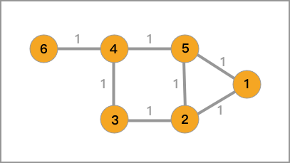
The adjacency matrix is:

\[\begin{split}A= \left(\begin{array}{rrrrrr} 0 & 1 & 0 & 0 & 1 & 0\\ 1 & 0 & 1 & 0 & 1 & 0\\ 0 & 1 & 0 & 1 & 0 & 0\\ 0 & 0 & 1 & 0 & 1 & 1\\ 1 & 1 & 0 & 1 & 0 & 0\\ 0 & 0 & 0 & 1 & 0 & 0\\ \end{array}\right) \end{split}\]

The degree matrix is:

\[\begin{split}D= \left(\begin{array}{rrrrrr} 2 & 0 & 0 & 0 & 0 & 0\\ 0 & 3 & 0 & 0 & 0 & 0\\ 0 & 0 & 2 & 0 & 0 & 0\\ 0 & 0 & 0 & 3 & 0 & 0\\ 0 & 0 & 0 & 0 & 3 & 0\\ 0 & 0 & 0 & 0 & 0 & 1\\ \end{array}\right) \end{split}\]

The Laplacian matrix is:

\[\begin{split}L = D - A = \left(\begin{array}{rrrrrr} 2 & -1 & 0 & 0 & -1 & 0\\ -1 & 3 & -1 & 0 & -1 & 0\\ 0 & -1 & 2 & -1 & 0 & 0\\ 0 & 0 & -1 & 3 & -1 & -1\\ -1 & -1 & 0 & -1 & 3 & 0\\ 0 & 0 & 0 & -1 & 0 & 1\\ \end{array}\right) \end{split}\]

32.8. Undirected Graph Cut

Currently, through the methods learned above, we can generate the undirected graph of the dataset and its corresponding Laplacian matrix.

You should be able to figure out that clustering is actually a process of seeking to cut the entire undirected graph into small pieces, and the small pieces cut out are each category (cluster). Therefore, the goal of spectral clustering is to divide the undirected graph into two or more subgraphs, making the nodes within the subgraphs similar and the nodes between the subgraphs different, so as to achieve the purpose of clustering.

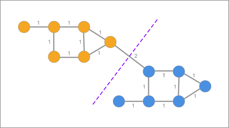
For the graph cut of the undirected graph \(G\), our goal is to cut the graph \(G(V, E)\) into \(k\) non - connected subgraphs. The set of vertices of each subgraph is \(A_1, A_2, \cdots, A_k\), which satisfy \(A_i \cap A_j=\varnothing\) and \(A_1\cup A_2\cup\cdots\cup A_k = V\).

For any two subsets of vertices \(A, B\subset V\) with \(A\cap B = \varnothing\), we define the cut - graph weight between \(A\) and \(B\) as:

\[ W(A, B) = \sum\limits_{i \in A, j \in B}w_{ij} \tag{10} \]

Then, for the set of \(k\) sub - graph vertices: \(A_1, A_2, \cdots, A_k\), the graph cut is defined as:

\[ cut(A_1,A_2,\cdots, A_k) = \frac 1 2 \sum\limits_{i=1}^{k}W(A_i, \overline{A}_i ) \tag{11} \]

where \(\overline{A}_i\) is the complement of \(A_i\), which means the union of the other subsets of \(V\) except the subset \(A_i\).

It is easy to see that \(cut(A_1,A_2,\cdots, A_k)\) describes the similarity between sub - graphs. The smaller its value, the greater the difference between sub - graphs. However, when dividing sub - graphs, formula (11) does not take into account the minimum number of nodes in a sub - graph, which easily leads to a single data point or very few data points being classified as an independent sub - graph, but this is obviously incorrect.

To approach this problem, we will introduce some regularization methods, among which the most commonly used ones are RatioCut and Ncut.

When performing RatioCut graph partitioning, it not only considers minimizing \(cut(A_1,A_2,\cdots, A_k)\), but also simultaneously considers maximizing the number of points in each sub - graph. Its definition is as follows:

\[ RatioCut(A_1,A_2,...A_k) = \sum\limits_{i=1}^{k}\frac{cut(A_i, \overline{A}_i )}{|A_i|} \tag{12} \]

Among them, \(|A_i|\) represents the number of nodes in the sub - graph \(A_i\).

Ncut graph partitioning is very similar to RatioCut graph partitioning, but it replaces the denominator \(|A_i|\) in RatioCut with \({assoc(A_i)}\). Since a large number of samples in a sub - graph does not necessarily mean a large weight, it is more in line with our goal to base the graph partitioning on weights. Therefore, generally speaking, Ncut graph partitioning is better than RatioCut graph partitioning.

\[ NCut(A_1,A_2,...A_k) = \sum\limits_{i=1}^{k}\frac{cut(A_i, \overline{A}_i )}{assoc(A_i, V)} \tag{13} \]

Among them, \({assoc(A_i, V)} = \sum_{V_j\in A_i}^{k} d_j\), where \(d_j = \sum_{i=1}^{n} w_{ji}\).

The derivation processes of Ncut graph partitioning and RatioCut graph partitioning are not explained for the time being because they are relatively complex.

32.9. Spectral Clustering Process and Implementation

After so much knowledge preparation above, let’s finally talk about the process of spectral clustering:

1. Construct an undirected graph \(G\) based on the data. Each node in the graph corresponds to a data point. Connect the similar points, and the weights of the edges are used to represent the similarity between the data.

2. Calculate the adjacency matrix \(A\) and degree matrix \(D\) of the graph, and solve the corresponding Laplacian matrix \(L\).

3. Find the first \(k\) eigenvalues \(\{\lambda\}_{i = 1}^k\) arranged in ascending order of \(L\) and the corresponding eigenvectors \(\{v\}_{i = 1}^k\).

4. Arrange the \(k\) eigenvectors together to form an \(N\times k\) matrix. Regard each row as a vector in the \(k\)-dimensional space, and use the K-Means algorithm for clustering to obtain the final clustering categories.

Looking at the above four steps, you will find that K-Means is still used at the end of spectral clustering. Then what is the essence of the spectral matrix?

In my opinion, the essence of spectral clustering is the K-Means clustering of the new matrix composed of its eigenvectors obtained through the Laplacian matrix transformation, and the Laplacian matrix transformation can be simply regarded as a process of dimensionality reduction.

The “spectrum” in spectral clustering actually refers to the general term for all eigenvectors in the matrix.

Next, we will implement spectral clustering using Python according to the spectral clustering process. First, generate a set of sample data. This time, we use make_circles() to generate circular data.

from sklearn import datasets
from matplotlib import pyplot as plt

%matplotlib inline

noisy_circles, _ = datasets.make_circles(
    n_samples=300, noise=0.1, factor=0.3, random_state=10
)

plt.scatter(noisy_circles[:, 0], noisy_circles[:, 1], color="b")

<matplotlib.collections.PathCollection at 0x1447bfdc0>

For this set of data, let’s try clustering it into two clusters using K-Means.

from sklearn.cluster import KMeans

plt.scatter(
    noisy_circles[:, 0],
    noisy_circles[:, 1],
    c=KMeans(n_clusters=2, n_init="auto").fit_predict(noisy_circles),
)

<matplotlib.collections.PathCollection at 0x1473c1d20>

As can be seen, the result is very unsatisfactory. So, we try to complete it through spectral clustering.

Referring to the spectral clustering process above, we know that first we need to calculate the adjacency matrix \(A\) of the undirected graph generated from the data. In this experiment, the K-nearest neighbor method is used to calculate the similarity weights corresponding to the edges in the undirected graph. The following is implemented through the knn_similarity_matrix(data, k) function:

import numpy as np


def knn_similarity_matrix(data, k):
    zero_matrix = np.zeros((len(data), len(data)))
    w = np.zeros((len(data), len(data)))

    for i in range(len(data)):
        for j in range(i + 1, len(data)):
            zero_matrix[i][j] = zero_matrix[j][i] = np.linalg.norm(
                data[i] - data[j]
            )  # 计算欧式距离

    for i, vector in enumerate(zero_matrix):
        vector_i = np.argsort(vector)
        w[i][vector_i[1 : k + 1]] = 1

    # 将两点间权重相加求平均
    w = (np.transpose(w) + w) / 2

    return w

Having obtained the adjacency matrix \(A\), we can calculate the degree matrix \(D\) and the corresponding Laplacian matrix \(L\), thus implementing the entire spectral clustering method:

def spectral_clustering(data, k, n):
    # 计算近邻矩阵、度矩阵、拉普拉斯矩阵
    A_matrix = knn_similarity_matrix(data, k)
    D_matrix = np.diag(np.power(np.sum(A_matrix, axis=1), -0.5))
    L_matrix = np.eye(len(data)) - np.dot(np.dot(D_matrix, A_matrix), D_matrix)

    # 计算特征值和特征向量
    eigvals, eigvecs = np.linalg.eig(L_matrix)

    # 选择前 n 个最小的特征向量
    indices = np.argsort(eigvals)[:n]
    k_eigenvectors = eigvecs[:, indices]
    k_eigenvectors

    # 使用 K-Means 完成聚类
    clusters = KMeans(n_clusters=n, n_init="auto").fit_predict(k_eigenvectors)

    return clusters

In the above algorithm implementation process, instead of using \(L = D - A\) to calculate the Laplacian matrix, we used the symmetric normalized Laplacian:

\[ {\displaystyle L^{\text{sym}}:=D^{-{\frac {1}{2}}}LD^{-{\frac {1}{2}}}=I-D^{-{\frac {1}{2}}}AD^{-{\frac {1}{2}}}} \tag{14} \]

Finally, we define the parameter k = 5 and cluster the data into two classes.

sc_clusters = spectral_clustering(noisy_circles, k=5, n=2)
sc_clusters

array([0, 0, 0, 1, 1, 1, 0, 0, 1, 1, 1, 0, 1, 1, 1, 0, 1, 1, 1, 1, 0, 1,
       0, 0, 1, 0, 0, 1, 1, 0, 0, 1, 0, 1, 1, 1, 1, 0, 1, 0, 0, 1, 1, 0,
       1, 1, 0, 0, 0, 0, 1, 0, 1, 0, 1, 1, 1, 0, 1, 0, 0, 0, 1, 0, 1, 0,
       0, 0, 0, 1, 1, 0, 0, 1, 1, 1, 1, 1, 1, 0, 1, 0, 0, 1, 0, 1, 0, 1,
       1, 0, 1, 0, 1, 1, 1, 0, 0, 1, 0, 1, 1, 1, 1, 1, 0, 1, 0, 0, 1, 1,
       0, 0, 1, 0, 1, 1, 0, 0, 0, 0, 1, 1, 0, 0, 1, 1, 1, 1, 1, 0, 0, 1,
       0, 1, 1, 1, 1, 0, 0, 1, 1, 0, 0, 0, 1, 0, 0, 0, 0, 0, 0, 0, 1, 1,
       1, 1, 1, 1, 0, 1, 0, 0, 1, 1, 1, 1, 1, 1, 0, 1, 1, 0, 0, 0, 0, 1,
       1, 1, 1, 0, 0, 0, 0, 1, 0, 1, 0, 0, 1, 1, 0, 1, 0, 1, 0, 0, 0, 1,
       1, 1, 0, 1, 0, 1, 0, 1, 0, 0, 1, 0, 0, 1, 0, 0, 0, 0, 0, 1, 1, 1,
       1, 0, 1, 0, 0, 0, 1, 0, 1, 1, 1, 1, 0, 0, 0, 1, 1, 0, 0, 0, 1, 1,
       1, 0, 0, 1, 0, 0, 1, 0, 1, 0, 0, 0, 1, 0, 1, 1, 0, 0, 0, 0, 1, 1,
       1, 0, 1, 1, 0, 1, 0, 0, 0, 0, 0, 1, 0, 1, 0, 0, 1, 1, 1, 1, 0, 0,
       0, 0, 1, 0, 0, 1, 0, 0, 1, 1, 0, 0, 0, 1], dtype=int32)

Visualizing the dataset according to the clustering labels, we can see that the effect of spectral clustering is very good.

plt.scatter(noisy_circles[:, 0], noisy_circles[:, 1], c=sc_clusters)

<matplotlib.collections.PathCollection at 0x147422cb0>

32.10. Spectral Clustering in scikit-learn

scikit-learn also provides an implementation of spectral clustering, specifically sklearn.cluster.SpectralClustering():

sklearn.cluster.SpectralClustering(n_clusters=8, eigen_solver=None, random_state=None, n_init=10, gamma=1.0, metric='rbf', n_neighbors=10, eigen_tol=0.0, assign_labels='kmeans', degree=3, coef0=1, kernel_params=None, n_jobs=1)

Its main parameters are:

- n_clusters: The number of clusters.
- eigen_solver: The eigenvalue solver.
- gamma: The kernel coefficient when using the kernel function for affinity.
- affinity: The method for calculating the adjacency matrix, which can choose kernel functions, k-nearest neighbors, etc.
- n_neighbors: The value of k when using the k-nearest neighbor method for the adjacency matrix selection.
- assign_labels: The final clustering method, defaulting to K-Means.

Spectral clustering is often used for image segmentation. So below we will try to use the scikit-learn implementation of spectral clustering to complete an interesting example. This example is referenced from the scikit-learn official documentation.

First, we need to generate a sample image with several circles of different sizes and noise.

# 生成 100px * 100px 的图像
l = 100
x, y = np.indices((l, l))
# 在图像中添加 4 个圆
center1 = (28, 24)
center2 = (40, 50)
center3 = (67, 58)
center4 = (24, 70)
radius1, radius2, radius3, radius4 = 16, 14, 15, 14
circle1 = (x - center1[0]) ** 2 + (y - center1[1]) ** 2 < radius1**2
circle2 = (x - center2[0]) ** 2 + (y - center2[1]) ** 2 < radius2**2
circle3 = (x - center3[0]) ** 2 + (y - center3[1]) ** 2 < radius3**2
circle4 = (x - center4[0]) ** 2 + (y - center4[1]) ** 2 < radius4**2

img = circle1 + circle2 + circle3 + circle4
mask = img.astype(bool)
img = img.astype(float)
# 添加随机噪声点
img += 1 + 0.2 * np.random.randn(*img.shape)

plt.figure(figsize=(5, 5))
plt.imshow(img)

<matplotlib.image.AxesImage at 0x14746bbe0>

Next, we use the spectral clustering method to complete image edge detection and obtain the processed image.

from sklearn.feature_extraction import image
from sklearn.cluster import spectral_clustering

graph = image.img_to_graph(img, mask=mask)  # 图像处理为梯度矩阵
graph.data = np.exp(-graph.data / graph.data.std())  # 正则化

labels = spectral_clustering(graph, n_clusters=4)
label_im = -np.ones(mask.shape)
label_im[mask] = labels

plt.figure(figsize=(5, 5))
plt.imshow(label_im)

<matplotlib.image.AxesImage at 0x14746beb0>

32.11. Advantages of Spectral Clustering

Spectral clustering evolved from graph theory and is a clustering method with a simple principle and good results. Compared with K-Means, spectral clustering mainly has the following advantages.

1. Suitable for clustering data distributions of various shapes.

2. Faster in calculation speed, especially significantly superior to other algorithms on large datasets.

3. Avoids the phenomenon that K-Means would classify a few outliers into one cluster.

D. Cai et al. DOI: 10.1109/TKDE.2005.198 once tested the clustering accuracy performance of spectral clustering and K-Means on the TDT2 and Reuters-21578 benchmark clustering datasets, and the results are as follows:

	TDT2		Reuters-21578
k value	K-Means	Spectral Clustering	K-Means	Spectral Clustering
2	0.989	0.998	0.871	0.923
3	0.974	0.996	0.775	0.816
4	0.959	0.996	0.732	0.793
…	…	…	…	…
9	0.852	0.984	0.553	0.625
10	0.835	0.979	0.545	0.615

It can be seen that the performance of spectral clustering is generally better than that of K-Means.

Of course, spectral clustering also has some disadvantages. For example, since K-Means clustering is used finally, the number of clusters needs to be specified in advance. Additionally, when using K-nearest neighbors to generate the adjacency matrix, the number of nearest neighbor samples also needs to be specified, and it is relatively sensitive to parameters.

Finally, we will briefly introduce several clustering methods that were not mentioned earlier.

32.12. Affinity Propagation Clustering

The English name of Affinity Propagation Clustering is Affinity Propagation. Affinity Propagation is designed based on the concept of message passing among data points. Different from clustering algorithms such as K-Means, Affinity Propagation Clustering also does not require determining the number of clusters in advance, that is, the K value. However, due to the low running efficiency of Affinity Propagation, it is not very suitable for clustering large datasets.

scikit-learn provides an implementation class for Affinity Propagation:

sklearn.cluster.AffinityPropagation(damping=0.5, max_iter=200, convergence_iter=15, copy=True, preference=None, metric='euclidean', verbose=False)

Its main parameters are:

- damping: Damping factor to avoid numerical oscillations.
- max_iter: Maximum number of iterations.
- affinity: Affinity evaluation method, default is Euclidean distance.

• You can view the Affinity Propagation paper, use cases, and source code through this page.

32.13. Mean Shift

Mean Shift is also known as mean shift clustering. The purpose of mean shift clustering is to find the densest regions and is also an iterative process. During the clustering process, first calculate the shifted mean of the initial center point, move this point to this shifted mean, and then use this as the new starting point to continue moving until the final conditions are met. Mean Shift also introduces a kernel function to improve the clustering effect. In addition, Mean Shift also has good applications in fields such as image segmentation and video tracking.

scikit-learn provides an implementation class for MeanShift:

MeanShift(bandwidth=None, seeds=None, bin_seeding=False, min_bin_freq=1, cluster_all=True, n_jobs=1)

32.14. Clustering Method Selection

In the content of this chapter, we introduced nearly ten different clustering algorithms. Among them, there are the classic K-Means, the efficient MiniBatchKMeans, the hierarchical and density clustering that do not require specifying the number of clusters, and the spectral clustering suitable for image segmentation. For these algorithms, how should we choose in practical applications? The following gives a reference diagram provided by scikit-learn:

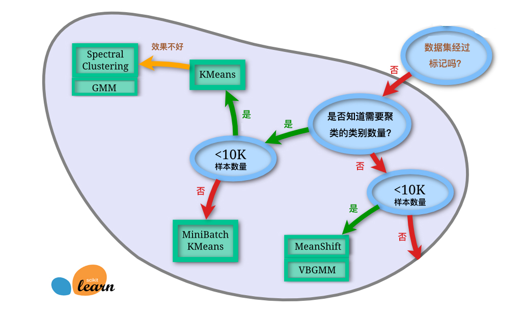
Of course, the above figure is only for reference. Facing the complex situations in practical applications, it still needs to be determined according to the specific circumstances.

32.15. Summary

This experiment mainly introduced the spectral clustering algorithm. In fact, spectral clustering is very common in practical applications, but its major drawback is that it is not suitable for large-scale data because calculating the eigenvalues and eigenvectors of the matrix is very time-consuming. The affinity propagation and Mean Shift clustering introduced at the end will be briefly mentioned, because these two algorithms actually do not have obvious advantages compared to the clustering algorithms we introduced earlier.

Related Links

• Spectral clustering - Wikipedia

---

○ Sharethis article link to your social media, blog, forum, etc. More external links will increase the search engine ranking of this site.

If you find this content helpful, you can buy me a coffee

Previous

31. Density Clustering to Mark Abnormal Shared Bicycles

Next

33. Comparative Evaluation of Common Clustering Algorithms