
28. Principal Component Analysis Principle and Applications#
28.1. Introduction#
In multivariate statistical analysis, principal components analysis (PCA) is a technique for analyzing and simplifying datasets. It is often used to reduce the dimensionality of a dataset while retaining the features that contribute the most to the variance in the dataset. PCA is also a very commonly used dimensionality reduction technique, and its essence can also be regarded as mapping the data while maximizing the retention of the original data. This experiment will dissect this technique, starting from basic mathematical knowledge and gradually delving deeper into the method.
28.2. Key Points#
Basis of vectors
Vector mapping
Variance and covariance
Eigenvalues and eigenvectors
Calculation of principal component analysis
28.3. Basis of Vectors#
You must be familiar with the term “vector”. As shown in the figure below, in a two-dimensional Cartesian coordinate system, how do you define vector \(A\)?
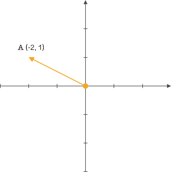
\(A(-2, 1)\) This should be the result that everyone comes up with. That’s right, we usually define it this way in high school. But in linear algebra, there will be another concept: basis.
A basis is also called a base, which is a fundamental tool for describing and characterizing vector spaces. A basis of a vector space is a special subset of it, and the elements of the basis are called basis vectors. Any element in a vector space can be uniquely represented as a linear combination of basis vectors. Using a basis can conveniently describe a vector space.
Therefore, a vector cannot be completely described solely by the coordinates of its endpoint. By introducing basis vectors, this problem can be accurately described. Usually, our descriptions implicitly introduce a definition: using the basis vectors \((1,0)\) and \((0,1)\) with a length of 1 in the positive directions of the \(x\) and \(y\) axes as the standard. At this time, the projection of vector \(A\) on the \(x\)-axis is 2, and the projection on the \(y\)-axis is 1. Then, by determining the direction of the basis vectors, the expression is \((-2,1)\).
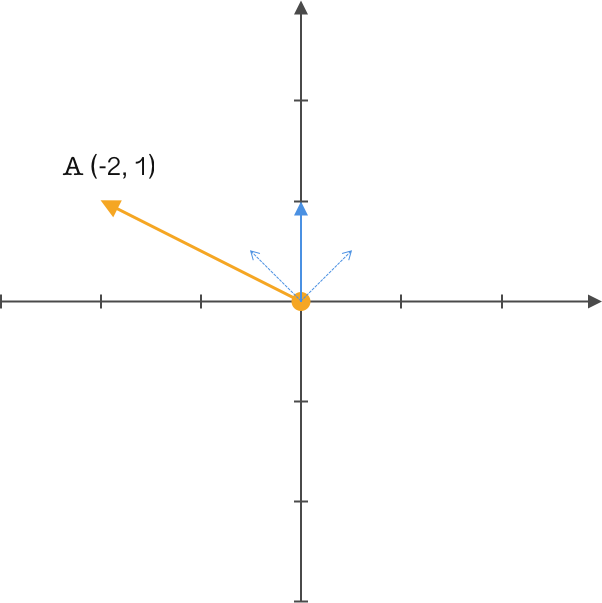
In the above picture and description, we defaultly choose the pair of orthogonal basis vectors \((1,0)\) and \((0,1)\) on the \(x\)- and \(y\)-axes with a length of 1, just for the convenience of corresponding to two-dimensional coordinates. In fact, any two linearly independent vectors can be used as a set of bases. Therefore, we get a conclusion: First, determine a set of bases in the space, and second, the accurate description of the vector is obtained by expressing the projection of the vector on the lines where the bases lie.
28.4. Redefine Vectors#
Currently, we know that any set of bases in space can redefine or describe a vector. Next, let’s take an example.
同样我们使用上面的 \(A\) 向量,但我们改变原来的基为 \((1,1)\) 和 \((-1,1)\) 。前面提到过,一般都喜欢将基的模长定义为 1,因为这样能简化运算,向量乘基直接就能得到新基上的坐标,所以我们标准化这组基的模长为 1,得到 \((\frac{\sqrt{2}}{2},\frac{\sqrt{2}}{2})\) 和 \((\frac{-\sqrt{2}}{2},\frac{\sqrt{2}}{2})\) 。很简单的转换,只需要对原来基的模做运算即可。
Similarly, we use the above vector \(A\), but we change the original basis to \((1,1)\) and \((-1,1)\). As mentioned before, it is generally preferred to define the norm of the basis as 1 because this simplifies the calculations and multiplying the vector by the basis directly gives the coordinates in the new basis. So we normalize the norm of this set of bases to 1, obtaining \((\frac{\sqrt{2}}{2},\frac{\sqrt{2}}{2})\) and \((\frac{-\sqrt{2}}{2},\frac{\sqrt{2}}{2})\). It is a very simple transformation and only requires operations on the norms of the original basis.
通过简单的变换现在我们得到了一组新基,并且模长为 \(1\),接下来就可以通过这组基来重新定义向量 \(A\) 了。如何转换 \(A\) 向量呢?平移还是旋转,下面我们通过简单的矩阵运算角度来认识这个问题。
Through simple transformation, we now obtain a new set of bases with a norm of 1. Next, we can redefine vector \(A\) using this set of bases. How to transform vector \(A\)? Translation or rotation? Next, we will understand this problem from the perspective of simple matrix operations.
我们将基按照行排列成矩阵,将向量按照列排列成矩阵,做矩阵的乘法得到一个新矩阵,此时矩阵中的 \((-\frac{\sqrt{2}}{2},\frac{3\sqrt{2}}{2})\) 便是向量 \(A\) \((-2,1)\) 在基 \((\frac{\sqrt{2}}{2},\frac{\sqrt{2}}{2})\) 和 \((\frac{-\sqrt{2}}{2},\frac{\sqrt{2}}{2})\) 上的新定义。
We arrange the bases as a matrix by rows and the vector as a matrix by columns, and perform matrix multiplication to obtain a new matrix. At this time, \((-\frac{\sqrt{2}}{2},\frac{3\sqrt{2}}{2})\) in the matrix is the new definition of vector \(A\) \((-2,1)\) in the bases \((\frac{\sqrt{2}}{2},\frac{\sqrt{2}}{2})\) and \((\frac{-\sqrt{2}}{2},\frac{\sqrt{2}}{2})\).
你应该会有这样的疑问,为什么基于向量做矩阵运算就能得到向量在新基上的重新定义?下面我们就来简单探讨一下这个问题。
You should have such a question: Why can we obtain the redefinition of a vector in a new basis by performing matrix operations on the vector? Now let’s briefly explore this issue.
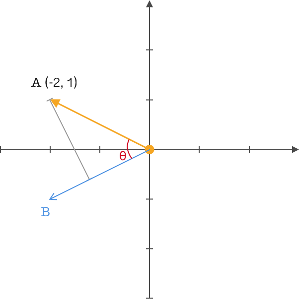
我们在向量 \(A\) 的图中再定义了一个向量 \(B\),并从向量 \(A\) 做投影到向量 \(B\) ,两个向量之间的夹角为 \(θ\),同时对它们做内积运算,得到一个熟悉的公式:
We defined another vector \(B\) in the diagram of vector \(A\), projected vector \(A\) onto vector \(B\), the angle between the two vectors is \(θ\), and at the same time performed an inner product operation on them, obtaining a familiar formula:
关键的地方来了,前面我们一直强调将基的模长取值为 \(1\),从而便于转换定义,这里我们就来实际运用一下。设置向量 \(B\) 的模长为 \(1\),那么上面的公式就可以变为:
Here comes the crucial part. We have been emphasizing that the magnitude of the basis is set to 1 for easier conversion of definitions. Now let’s put it into actual use. Set the magnitude of vector \(B\) to 1, then the above formula can be transformed into:
此时可以得到一个结论:两个向量相乘,且其中一个模长为 \(1\),那么结果就是该向量在另一个向量上投影的矢量距离。
At this point, we can draw a conclusion: when two vectors are multiplied and the magnitude of one of them is 1, then the result is the vector distance of the projection of this vector onto the other vector.
现在转换到上面的内容就一目了然了,向量 \(B\) 模长为 \(1\),与我们定义的新基一致,由于只有一个基,所以不存在线性关系,通过向量 \(A\) 与该组基做矩阵运算最终便得到了新的映射。
Now it becomes clear when we switch to the above content. The magnitude of vector \(B\) is 1, which is consistent with the new basis we defined. Since there is only one basis, there is no linear relationship. By performing matrix operations on vector \(A\) and this set of bases, we finally obtain a new mapping.
28.5. Redefine the Matrix#
前面使用不同的基,实现了对向量的重新映射,同样通过一个简单的矩阵运算来说明了这个问题。下面我们接着引入一些新知识对矩阵也做定义。 Previously, by using different bases, we achieved a re - mapping of vectors, and this issue was also illustrated through a simple matrix operation. Next, we will introduce some new knowledge to define matrices as well.
我们通过一组新基重新映射了一个向量,若此时有多个向量又该如何映射?当然还是可以通过矩阵来轻松搞定,下面使用一组基来映射多个向量: We remapped a vector through a new set of bases. What if there are multiple vectors at this time? Of course, it can still be easily done through matrices. Next, we use a set of bases to map multiple vectors:
在基不变的情况下,我们增加了三个按列排列的二维向量。可以看到,矩阵帮助我们快速的将原来按 \((1,0)\) 和 \((0,1)\) 定义的向量全部映射到 \((\frac{\sqrt{2}}{2},\frac{\sqrt{2}}{2})\) 和 \((\frac{-\sqrt{2}}{2},\frac{\sqrt{2}}{2})\) 上 With the basis remaining unchanged, we added three two - dimensional vectors arranged by columns. It can be seen that the matrix helps us quickly map all the vectors originally defined by \((1, 0)\) and \((0, 1)\) to \((\frac{\sqrt{2}}{2},\frac{\sqrt{2}}{2})\) and \((\frac{-\sqrt{2}}{2},\frac{\sqrt{2}}{2})\).
这里简单的解释下上面三个矩阵的含义,第一个矩阵表示将两个基按行排列;第二个矩阵表示将四个向量按列排列;第三个矩阵表示将第二个矩阵作用到第一个矩阵所在基的新映射,此时每一列对应第二个矩阵的每一列。 Here is a simple explanation of the meaning of the above three matrices. The first matrix represents arranging two bases by rows; the second matrix represents arranging four vectors by columns; the third matrix represents applying the second matrix to the new mapping of the basis where the first matrix lies, and at this time each column corresponds to each column of the second matrix.
除此之外,与之对应的改变基的数量,我们来看看结果如何: In addition, corresponding to changing the number of bases, let’s see what the result is:
可以发现在增加了一个基后,原来的二维向量映射成了一个三维向量。是不是有种恍然大悟的感觉,改变基的数量就可以改变向量的维数,那么同样如果减少基的数量为 \(1\),向量就会减少维数。似乎这里与我们的主题降维就有了一点关联了。 It can be found that after adding a basis, the original two - dimensional vector is mapped into a three - dimensional vector. Does it give you a feeling of sudden realization? Changing the number of bases can change the dimension of the vector. Similarly, if the number of bases is reduced to 1, the dimension of the vector will be reduced. It seems that there is a certain connection here with our topic of dimensionality reduction.
下面将矩阵升高维度,使用 \(i\) 个 \(k\) 维的 \(M\) 向量矩阵与 \(j\) 个 \(k\) 维的 \(N\) 向量矩阵做运算,通过数学方式做下面定义: Next, raise the dimension of the matrix. Perform operations on an \(i\times k\) matrix of \(M\) vectors and a \(j\times k\) matrix of \(N\) vectors, and make the following definitions in a mathematical way:
结合上面我们的结论来分析该表达式,可以看出我们将 \(j\) 个按列组成的向量映射到了 \(i\) 个按行排列的基中得到一个 \(i\) 行 \(j\) 列的矩阵。此时减小 \(i\) 的取值也就是减少了基的数量,矩阵运算便后得到相对低维映射的矩阵。这里通过高维函数表达式再次验证了基的数量决定了向量映射后的维数。 Combining the above conclusions to analyze this expression, it can be seen that we map \(j\) column - formed vectors into \(i\) row - arranged bases to obtain an \(i\times j\) matrix. At this time, reducing the value of \(i\) means reducing the number of bases, and after matrix operations, a matrix with a relatively lower - dimensional mapping is obtained. Here, through the high - dimensional function expression, it is verified again that the number of bases determines the dimension of the vector after mapping.
28.6. Principal Component Analysis (PCA)#
做了这么多的铺垫,终于到了本实验的核心问题。通过前面的叙述我们已经知道了基的个数决定着向量映射后的维数。所以问题得到了转换,现在需要做的就是找到最优并且数量合适的基。 After so much groundwork, we finally come to the core problem of this experiment. From the previous narrative, we already know that the number of bases determines the dimension of the vector after mapping. So the problem has been transformed, and what we need to do now is to find the optimal and appropriately - numbered bases.
还记得实验开头对主成分分析的描述吗?「保持数据集中的对方差贡献最大的特征」这是主成分分析使用的一个特点也是要求。在对方差理解前我们先从为什么需要引入方差开始说明。 Do you still remember the description of principal component analysis (PCA) at the beginning of the experiment? “Retain the features in the dataset that contribute the most to the variance” This is both a characteristic and a requirement of PCA. Before understanding variance, let’s first explain why variance needs to be introduced.
在二维空间中有如下图中的一些数据点: There are some data points in the two - dimensional space as shown in the following figure:
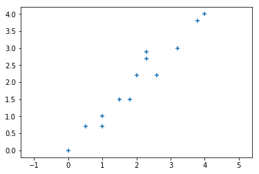
可以看到数据点的 \(x\) 与 \(y\) 之间的相关性很强,所以数据就会出现冗余。我们可以对该数据进行降维处理,也就是降到一维,通过一个维度来表现该二维数据。 It can be seen that there is a strong correlation between the \(x\) and \(y\) of the data points, so there is data redundancy. We can perform dimensionality reduction on this data, that is, reduce it to one dimension, and represent this two - dimensional data through one dimension.
现在你应该能联想到若选择一个最优基与该二维数据做矩阵运算,便可实现降维。关于基的选择,其实比较直观想到的就是在一、三象限之间的对角线。为什么会有这个想法,因为使用该基来映射数据数据点后看起来和原来最数据点分布最相近,同时投影也使得数据点最分散,即投影后的数据的方差最大,这样降维的同时也最大化的保留原始数据的信息。 Now you should be able to associate that if you choose an optimal basis and perform matrix operations on this two - dimensional data, dimensionality reduction can be achieved. Regarding the choice of basis, what comes to mind intuitively is actually the diagonal line between the first and third quadrants. Why do we have this idea? Because after using this basis to map the data points, it looks most similar to the original data point distribution. At the same time, the projection also makes the data points the most dispersed, that is, the variance of the projected data is the largest. In this way, while reducing the dimension, the information of the original data is retained to the maximum extent.
若使用 \(x\) 或 \(y\) 轴进行投影,可以清楚的观察到很多点在投影后会重合,相当于数据的丢失,这也是为什么投影要最分散的原因。 If we use the \(x\) - axis or \(y\) - axis for projection, it can be clearly observed that many points will coincide after projection, which is equivalent to data loss. This is also the reason why the projection should be the most dispersed.
下面通过代码来演示降维的操作,首先加载上面的数据点: The following demonstrates the dimensionality reduction operation through code. First, load the above data points:
import numpy as np
import matplotlib.pyplot as plt

%matplotlib inline

x = np.array([0, 0.5, 1, 1, 1.5, 1.8, 2, 2.3, 2.3, 2.6, 3.2, 3.8, 4])
y = np.array([0, 0.7, 1, 0.7, 1.5, 1.5, 2.2, 2.9, 2.7, 2.2, 3, 3.8, 4])

arr = np.array([x, y])
plt.axis("equal")
plt.scatter(x, y, marker="+")
<matplotlib.collections.PathCollection at 0x12867cc70>

直观上我们选择一象限副对角线作为基,并且标准化模长为 \(1\),最终为 \((\frac{\sqrt{2}}{2},\frac{\sqrt{2}}{2})\) 。 Intuitively, we choose the secondary diagonal line in the first quadrant as the basis and normalize the modulus length to 1, which is ultimately \((\frac{\sqrt{2}}{2},\frac{\sqrt{2}}{2})\).
base = np.array([np.sqrt(2) / 2, np.sqrt(2) / 2])  # 基向量
base
array([0.70710678, 0.70710678])
接着就是做两者的矩阵运算,得到降维后的数据。 Next is to perform matrix operations on the two to obtain the data after dimensionality reduction.
result_eye = np.dot(base, arr)
result_eye
array([0.        , 0.84852814, 1.41421356, 1.20208153, 2.12132034,
       2.33345238, 2.96984848, 3.67695526, 3.53553391, 3.39411255,
       4.38406204, 5.37401154, 5.65685425])
现在,我们得到了降维后的一维数组。由于一维数组无法在二维平面可视化,所以这里也无法与原数据进行可视化对比。 Now, we have obtained the one - dimensional array after dimensionality reduction. Since a one - dimensional array cannot be visualized in a two - dimensional plane, it is also impossible to make a visual comparison with the original data here.
前面,我们通过肉眼观察数据非分布趋势来选择降维的基,效果还不错。但如果原始数据的维数很大超过二维空间,无法观察数据分布该如何选择基呢?所以,接下来还需要继续探讨。 Previously, we selected the basis for dimensionality reduction by visually observing the non - distribution trend of the data, and the effect was quite good. However, if the dimensionality of the original data is very large and exceeds two - dimensional space, and it is impossible to observe the data distribution, how should we choose the basis? Therefore, further exploration is still needed next.
28.7. Variance and Covariance#
统计学中,方差是用来度量单个随机变量的离散程度。也就是说,最大方差给出了数据最重要的信息。如上面的例子,数据点投影后投影值尽可能分散,而这种分散程度,可以用数学上的方差来表述。一个维度中的方差,可以看作是该维度中每个元素与其均值的差平方和的均值,公式如下: In statistics, variance is used to measure the dispersion of a single random variable. That is to say, the maximum variance gives the most important information of the data. As in the above example, after the data points are projected, the projected values are as scattered as possible, and this degree of scattering can be expressed by variance in mathematics. The variance in one dimension can be regarded as the mean of the sum of the squares of the differences between each element in that dimension and its mean. The formula is as follows:
因此,我们的目标变成: Therefore, our goal becomes:
Find a basis, map the original two-dimensional data points through this basis, and obtain a result with the maximum variance, so as to achieve the purpose of dimensionality reduction.
上面二维降成一维时,我们寻找使得该数据集最大方差的一个基,容易联想到从更高维降到低维时,步骤应该是先寻找第一个最大方差的基,接着寻找第二个次大方差的基,依次找到相应维数的基的数量。 When reducing from two dimensions to one dimension above, we look for a basis that maximizes the variance of the data set. It is easy to think that when reducing from higher dimensions to lower dimensions, the steps should be to first find the basis with the largest variance, then find the basis with the second largest variance, and so on until the number of bases corresponding to the appropriate dimension is found.
想法看似符合逻辑,但实际上是有问题的。单纯这样选择会使得后面一个基的方向与前面一个基的方向几乎重合,这样得到的维度是没有意义的。所以限制条件来了,在不断寻找最大方差基的同时,我们需要两个基之间是没有相关性的,也就是两者独立,这样获得的基之间是没有重复性的。 The idea seems logical, but in fact there is a problem. Making such a choice simply will cause the direction of the latter basis to almost coincide with that of the former basis, and the resulting dimension is meaningless. So the constraint comes. While continuously looking for the basis with the largest variance, we need the two bases to be uncorrelated, that is, independent of each other, so that the obtained bases have no repetition.
如何才能使得两个向量之间独立?在二维空间中两个向量垂直,则线性无关,那么在高维空间中,向量之间相互正交,则线性无关。 How can we make two vectors independent? In a two-dimensional space, if two vectors are perpendicular, they are linearly independent. Then in a high-dimensional space, if vectors are orthogonal to each other, they are linearly independent.
接着我们深入方差,方差其实是一种特殊的结构,可以看到上面的公式中两个变量相同都是 \((X_{i}-\bar{X})\) ,用来衡量两个相同变量的误差,那如果两个变量不同呢?我们变换变量 \((X_{i}-\bar{X})\) 为 \((Y_{i}-\bar{Y})\) ,那方差公式就变成了: Next, we delve into variance. Variance is actually a special structure. As can be seen in the formula above, the two variables are the same, both \((X_{i}-\bar{X})\), which is used to measure the error between two identical variables. What if the two variables are different? We transform the variable \((X_{i}-\bar{X})\) into \((Y_{i}-\bar{Y})\), and then the variance formula becomes:
可以得到:\(cov(x,x) = var(x)\) It can be obtained that: \(cov(x,x) = var(x)\)
实际上这个叫协方差,协方差一般用来刻画两个随机变量的相似程度。也就是从原来衡量两个相同变量的误差,到现在变成了衡量两个不同变量的误差。通俗点可以理解为:两个变量在变化过程中是否同向变化?还是反方向变化?同向或反向程度如何? Actually, this is called covariance, which is generally used to describe the similarity between two random variables. That is, it has changed from originally measuring the error between two identical variables to now measuring the error between two different variables. To put it simply, it can be understood as: Do the two variables change in the same direction during the change process? Or in the opposite direction? And to what extent do they change in the same or opposite directions?
好巧,似乎协方差就能表述两个向量之间的相关性,按照前面选择基的要求时需要基之间相互正交,那么让两个变量之间的协方差等于 \(0\) 不就可以了吗?因此,选择时让下一个基与上一个基之间的协方差等于 \(0\),那么得到的两个基必然是相互正交的。 Coincidentally, it seems that covariance can represent the correlation between two vectors. According to the previous requirement for choosing bases, the bases need to be orthogonal to each other. So, wouldn’t it be okay to make the covariance between two variables equal to 0? Therefore, when choosing, make the covariance between the next base and the previous base equal to 0, and then the two resulting bases must be orthogonal to each other.
28.8. Covariance Matrix#
上一段内容我们通过方差到协方差已经了解并解决了如何选择正交基,从而达到降维的要求。可是从协方差的公式中又出现了新问题。协方差最多只能衡量两个变量之间的误差,如果有 \(n\) 个向量则需要计算 \(\frac{n!}{(n-2)!*2}\) 个协方差。因此我们继续扩展问题到多向量。通过协方差的定义来计算任意两个变量的关系: In the previous section, we have understood and solved how to choose orthogonal bases from variance to covariance to meet the requirement of dimensionality reduction. However, a new problem has emerged from the covariance formula. Covariance can only measure the error between two variables at most. If there are \(n\) vectors, then \(\frac{n!}{(n - 2)! * 2}\) covariances need to be calculated. Therefore, we continue to expand the problem to multiple vectors. Calculate the relationship between any two variables through the definition of covariance:
下面,我们以向量个数等于 \(3\) 为例,我们转变为矩阵的表示形式: Next, taking the number of vectors equal to 3 as an example, we transform it into the matrix representation:
从矩阵中会发现协方差矩阵其实就是由对角线的方差与非对角线的协方差构成,所以协方差矩阵的核心理解:由向量自身的方差与向量之间的协方差构成。这个定义延伸到更多向量时同样受用。 It can be found from the matrix that the covariance matrix is actually composed of the variances on the diagonal and the covariances on the non - diagonal. Therefore, the core understanding of the covariance matrix is: it is composed of the variances of the vectors themselves and the covariances between the vectors. This definition also applies when extended to more vectors.
所以协方差矩阵就是解决 PCA 问题的关键,终于问题又有了突破口。通过前面的讲解,现在问题可以简化为: Therefore, the covariance matrix is the key to solving the PCA problem, and finally there is a breakthrough in the problem. Through the previous explanations, the problem can now be simplified to:
选择一组基,使得原始向量通过该基映射到新的维度,同时需要满足使得该向量的方差最大,向量之间的协方差为 \(0\) ,也就是矩阵对角化。 Select a set of bases such that the original vectors are mapped to new dimensions through these bases. At the same time, it is necessary to satisfy that the variance of the vectors is maximized and the covariance between the vectors is 0, that is, matrix diagonalization.
28.9. Eigenvalues and Eigenvectors#
目前问题已经很浅显易懂了,首先得到向量数据的协方差矩阵,其次通过协方差矩阵对方差与协方差的处理获得用于降维的基。找到问题后,接下来就是如何解决问题了。 The problem is now quite straightforward. First, obtain the covariance matrix of the vector data. Second, through the processing of the variance and covariance by the covariance matrix, obtain the bases for dimensionality reduction. After identifying the problem, the next step is how to solve it.
再观察一下协方差矩阵,我们可以发现其实它是一个对称矩阵。在矩阵中对称矩阵有很多特殊的性质,例如,如果对其进行特征分解,那么就会得到两个概念:特征值与特征向量。由于是对称矩阵,所以特征值所对应的特征向量一定无线性关系,即相互之间一定正交,内积为零。 Looking at the covariance matrix again, we can find that it is actually a symmetric matrix. Symmetric matrices in matrices have many special properties. For example, if we perform eigen decomposition on it, we will get two concepts: Eigenvalues and Eigenvectors. Since it is a symmetric matrix, the eigenvectors corresponding to the eigenvalues must have no linear relationship, that is, they must be orthogonal to each other and the inner product is zero.
在线性代数中给定一个方阵 \(A\) ,它的特征向量 \(v\) 在 \(A\) 变换的作用下,得到的新向量仍然与原来的 \(v\) 保持在同一条直线上,且仅仅在尺度上变为原来的 \(\lambda\) 倍。则称 \(v\) 是 \(A\) 的一个特征向量,\(\lambda\) 是对应的特征值,即: In linear algebra, given a square matrix \(A\), for its eigenvector \(v\), under the action of the transformation of \(A\), the new vector obtained still lies on the same straight line as the original \(v\), and only changes by a factor of \(\lambda\) in scale. Then \(v\) is called an eigenvector of \(A\), and \(\lambda\) is the corresponding eigenvalue, that is:
这里的特征向量 \(v\) 也就是矩阵 \(A\) 的主成分,而 \(\lambda\) 则是其对应的权值也就是各主成分的方差大小。 The eigenvector \(v\) here is also the principal component of matrix \(A\), and \(\lambda\) is the corresponding weight, which is the variance magnitude of each principal component.
至此,我们的目的就是寻找主成分,所以问题就转变成了寻找包含主成分最多的特征向量 \(v\),但是这个 \(v\) 并不好直观的度量,由此我们可以转变为寻找与之对应的权值 \(\lambda\),\(\lambda\) 越大则所对应的特征向量包含的主成分也就越多,所以问题接着转变为了寻找最大值的特征值 \(\lambda\)。 So far, our goal is to find the principal components. Therefore, the problem has been transformed into finding the eigenvector \(v\) that contains the most principal components. However, this \(v\) is not easy to measure intuitively. Thus, we can transform it into finding the corresponding weight \(\lambda\). The larger \(\lambda\) is, the more principal components the corresponding eigenvector contains. So the problem then turns into finding the eigenvalue \(\lambda\) with the maximum value.
所以,问题基本上已经得到了解决: So, the problem has basically been solved:
通过计算向量矩阵得到其协方差矩阵,然后特征分解协方差矩阵得到包含主成分的特征向量与对应的特征值,最后通过特征值的大小排序后依次筛选出需要用于降维的特征向量个数。 Calculate the covariance matrix of a vector matrix, then perform eigen decomposition on the covariance matrix to obtain the eigenvectors containing the principal components and their corresponding eigenvalues. Finally, sort the eigenvalues by magnitude and sequentially select the number of eigenvectors required for dimensionality reduction.
在前面小节中我们选择了肉眼观察的一组基对二位数据进行降维,下面我们尝试利用协方差矩阵的思想来对同样的数据做降维处理。 In the previous section, we selected a set of bases observed by the naked eye to perform dimensionality reduction on two-dimensional data. Next, we will try to use the idea of the covariance matrix to perform dimensionality reduction on the same data.
首先求得协方差矩阵,通过NumPy的\(cov\)函数来实现 First, obtain the covariance matrix, which is achieved through the \(cov\) function in NumPy.
covMat = np.cov(arr)  # 计算协方差矩阵
covMat
array([[1.48      , 1.47      ],
       [1.47      , 1.54141026]])
接下来利用NumPy中的线性代数工具linalg特征分解协方差矩阵得到特征值、特征向量
Next, use the linear algebra tool
linalg
in NumPy to perform eigen decomposition on the covariance
matrix to obtain the eigenvalues and eigenvectors.
eigVal, eigVec = np.linalg.eig(np.mat(covMat))  # 获得特征值、特征向量
eigVal, eigVec
(array([0.04038448, 2.98102578]),
 matrix([[-0.71445199, -0.69968447],
         [ 0.69968447, -0.71445199]]))
然后,我们根据特征值来选择特征向量。对特征值降序排序,取第一个特征向量。 Then, we select the eigenvectors based on the eigenvalues. Sort the eigenvalues in descending order and take the first eigenvector.
eigValInd = np.argsort(-eigVal)  # 特征值降序排序
bestVec = eigVec[:, eigValInd[:1]]  # 取最好的一个特征向量
bestVec
matrix([[-0.69968447],
        [-0.71445199]])
最后,利用该特征向量对前面的示例数据降维,得到一维数据: Finally, use this eigenvector to reduce the dimensionality of the previous example data to obtain one-dimensional data:
result_cov = np.dot(arr.T, bestVec)
result_cov
matrix([[ 0.        ],
        [-0.84995863],
        [-1.41413646],
        [-1.19980086],
        [-2.12120469],
        [-2.33111003],
        [-2.97116331],
        [-3.68118505],
        [-3.53829465],
        [-3.39097399],
        [-4.38234627],
        [-5.37371854],
        [-5.65654583]])
现在,我们来绘制出通过最优特征向量和前面肉眼观察的一组基各自降维的结果。 Now, let’s plot the results of dimensionality reduction using the optimal eigenvector and a set of bases observed by the naked eye before.
fig, axes = plt.subplots(1, 2, figsize=(10, 5))
axes[0].scatter(result_cov.flatten().A[0], [0 for i in range(len(x))], marker="+")
axes[1].scatter(result_eye, [0 for i in range(len(x))], marker="+")
<matplotlib.collections.PathCollection at 0x1287a2650>

由于上面是一维数组的二维展示,我们看不出太多的信息。所以,下面通过度量两者的方差,比较谁更好: Since the above is a two-dimensional display of a one-dimensional array, we can’t see much information. Therefore, below, we compare which one is better by measuring the variances of the two:
np.var(result_cov), np.var(result_eye)
(2.7517161001590864, 2.751420118343195)
可以看到,通过分解协方差矩阵来降维得到结果的方差要大一点,这也就代表了保留的原始数据信息更多。看来,眼睛的确不如数学方法可靠。 It can be seen that the variance of the result obtained by reducing the dimensionality through decomposing the covariance matrix is a bit larger, which means that more original data information is retained. It seems that the eyes are indeed not as reliable as mathematical methods.
28.10. Dimensionality Reduction of High-Dimensional Data#
前面的例子中,为了便于教学只分析了二维数据降到一维的过程。下面,我们将对一个包含590个特征的数据集进行降维处理。 In the previous example, for the convenience of teaching, only the process of reducing two-dimensional data to one-dimensional was analyzed. Next, we will perform dimensionality reduction on a dataset containing 590 features.
\(590\) 个特征不算太多,但也是一个很大的维度了。所以,这里使用降维的方式处理数据集,得到一个维度更低,但仍然保留绝大部分的原始信息的新数据集。 590 features are not too many, but it is still a very large dimension. Therefore, here we use dimensionality reduction to process the dataset and obtain a new dataset with a lower dimension but still retaining most of the original information.
首先,通过下面的链接加载数据并预览数据集。 First, load the data and preview the dataset through the following link.
wget -nc https://cdn.aibydoing.com/aibydoing/files/pca_data.csv
import pandas as pd

df = pd.read_csv("pca_data.csv")
df.describe()
| 0 | 1 | 2 | 3 | 4 | 5 | 6 | 7 | 8 | 9 | ... | 580 | 581 | 582 | 583 | 584 | 585 | 586 | 587 | 588 | 589 | |
|---|---|---|---|---|---|---|---|---|---|---|---|---|---|---|---|---|---|---|---|---|---|
| count | 1567.000000 | 1567.000000 | 1567.000000 | 1567.000000 | 1567.000000 | 1567.0 | 1567.000000 | 1567.000000 | 1567.000000 | 1567.000000 | ... | 1567.000000 | 1567.000000 | 1567.000000 | 1567.000000 | 1567.000000 | 1567.000000 | 1567.000000 | 1567.000000 | 1567.000000 | 1567.000000 |
| mean | 3014.452896 | 2495.850231 | 2200.547318 | 1396.376627 | 4.197013 | 100.0 | 101.112908 | 0.121822 | 1.462862 | -0.000841 | ... | 0.005396 | 97.934373 | 0.500096 | 0.015318 | 0.003847 | 3.067826 | 0.021458 | 0.016475 | 0.005283 | 99.670066 |
| std | 73.480613 | 80.227793 | 29.380932 | 439.712852 | 56.103066 | 0.0 | 6.209271 | 0.008936 | 0.073849 | 0.015107 | ... | 0.001956 | 54.936224 | 0.003403 | 0.017174 | 0.003719 | 3.576891 | 0.012354 | 0.008805 | 0.002866 | 93.861936 |
| min | 2743.240000 | 2158.750000 | 2060.660000 | 0.000000 | 0.681500 | 100.0 | 82.131100 | 0.000000 | 1.191000 | -0.053400 | ... | 0.001000 | 0.000000 | 0.477800 | 0.006000 | 0.001700 | 1.197500 | -0.016900 | 0.003200 | 0.001000 | 0.000000 |
| 25% | 2966.665000 | 2452.885000 | 2181.099950 | 1083.885800 | 1.017700 | 100.0 | 97.937800 | 0.121100 | 1.411250 | -0.010800 | ... | 0.005396 | 91.549650 | 0.497900 | 0.011600 | 0.003100 | 2.306500 | 0.013450 | 0.010600 | 0.003300 | 44.368600 |
| 50% | 3011.840000 | 2498.910000 | 2200.955600 | 1287.353800 | 1.317100 | 100.0 | 101.492200 | 0.122400 | 1.461600 | -0.001300 | ... | 0.005396 | 97.934373 | 0.500200 | 0.013800 | 0.003600 | 2.757700 | 0.020500 | 0.014800 | 0.004600 | 72.023000 |
| 75% | 3056.540000 | 2538.745000 | 2218.055500 | 1590.169900 | 1.529600 | 100.0 | 104.530000 | 0.123800 | 1.516850 | 0.008400 | ... | 0.005396 | 97.934373 | 0.502350 | 0.016500 | 0.004100 | 3.294950 | 0.027600 | 0.020300 | 0.006400 | 114.749700 |
| max | 3356.350000 | 2846.440000 | 2315.266700 | 3715.041700 | 1114.536600 | 100.0 | 129.252200 | 0.128600 | 1.656400 | 0.074900 | ... | 0.028600 | 737.304800 | 0.509800 | 0.476600 | 0.104500 | 99.303200 | 0.102800 | 0.079900 | 0.028600 | 737.304800 |
8 rows × 590 columns
可以看到,数据集拥有1567个样本,每个样本拥有590个特征。 It can be seen that the dataset has 1567 samples, and each sample has 590 features.
在进行得到协方差矩阵处理前,我们会对数据按维度进行零均值化处理。其主要目的是去除均值对变换的影响,减去均值后数据的信息量没有变化,即数据的区分度(方差)是不变的。如果不去均值,第一主成分,可能会或多或少的与均值相关。前面的例子我们省略了这一步,是为了能更好的观察绘制出来的图像,且当时并无太大影响。 Before performing the operation to obtain the covariance matrix, we will zero-center the data by dimension. The main purpose is to remove the influence of the mean on the transformation. After subtracting the mean, the information content of the data remains unchanged, that is, the discriminability (variance) of the data remains the same. If the mean is not removed, the first principal component may be more or less related to the mean. In the previous example, we omitted this step in order to better observe the plotted images, and there was not much impact at that time.
data = df.values
mean = np.mean(data, axis=0)
data = data - mean
data
array([[ 1.64771044e+01,  6.81497692e+01, -1.28140177e+01, ...,
        -8.67361738e-17, -3.29597460e-17, -1.70530257e-13],
       [ 8.13271044e+01, -3.07102308e+01,  2.98748823e+01, ...,
         3.62509579e-03,  7.16666667e-04,  1.08534434e+02],
       [-8.18428956e+01,  6.40897692e+01, -1.41362177e+01, ...,
         3.19250958e-02,  9.51666667e-03, -1.68098663e+01],
       ...,
       [-3.56428956e+01, -1.16070231e+02,  5.75268229e+00, ...,
        -7.87490421e-03, -2.78333333e-03, -5.61469663e+01],
       [-1.19532896e+02,  3.61597692e+01, -2.35140177e+01, ...,
         8.02509579e-03,  2.21666667e-03, -6.17596635e+00],
       [-6.95328956e+01, -4.50902308e+01, -5.10291771e+00, ...,
        -2.74904215e-04, -7.83333333e-04,  3.81143337e+01]])
接下来,计算协方差矩阵: Next, calculate the covariance matrix:
covMat = np.cov(data, rowvar=False)
covMat
array([[ 5.39940056e+03, -8.47962623e+02,  1.02671010e+01, ...,
        -1.67440688e-02, -5.93197815e-03,  2.87879850e+01],
       [-8.47962623e+02,  6.43649877e+03,  1.35942679e+01, ...,
         1.21967287e-02,  2.32652705e-03,  3.37335304e+02],
       [ 1.02671010e+01,  1.35942679e+01,  8.63239193e+02, ...,
        -7.59126039e-03, -2.59521865e-03, -9.07023669e+01],
       ...,
       [-1.67440688e-02,  1.21967287e-02, -7.59126039e-03, ...,
         7.75231441e-05,  2.45865358e-05,  3.22979001e-01],
       [-5.93197815e-03,  2.32652705e-03, -2.59521865e-03, ...,
         2.45865358e-05,  8.21484994e-06,  1.04706789e-01],
       [ 2.87879850e+01,  3.37335304e+02, -9.07023669e+01, ...,
         3.22979001e-01,  1.04706789e-01,  8.81006310e+03]])
然后,分解协方差矩阵获得特征值与特征向量,同时绘制出前30个特征值变化曲线图。 Then, decompose the covariance matrix to obtain the eigenvalues and eigenvectors, and at the same time plot the curve of the first 30 eigenvalues.
eigVal, eigVec = np.linalg.eig(np.mat(covMat))
plt.plot(eigVal[:30], marker="o")
[<matplotlib.lines.Line2D at 0x12fe36230>]

可以看到方差的急剧下降,到后面绝大多数的主成分所占方差几乎为 \(0\),因此更说明了对该数据进行主成分分析的必要性。其中,第 4 个点是比较明显的拐点。 It can be seen that there is a sharp drop in variance, and for most of the subsequent principal components, the variance accounted for is almost \(0\), which further demonstrates the necessity of performing principal component analysis on this data. Among them, the 4th point is a relatively obvious inflection point.
这里,我们计算前 4 个主成分所占的方差数值与 90% 主成分的方差总和数值: Here, we calculate the variance values accounted for by the first 4 principal components and the total variance value of 90% of the principal components:
sum(eigVal[:4]), sum(eigVal) * 0.9
(85484127.2361191, 81131452.77696122)
观察两者的数值大小,可以发现在 590 个主成分中,前 4 个主成分所占的方差就已经超过了 90%。说明后 586 个主成分仅占 10% ,即仅用前 4 个特征向量来映射数据,就可以保留绝大多数的原始数据信息。 By observing the numerical magnitudes of the two, it can be found that among the 590 principal components, the variance accounted for by the first 4 principal components already exceeds 90%. This indicates that the remaining 586 principal components only account for 10%, meaning that by using only the first 4 eigenvectors to map the data, the vast majority of the original data information can be retained.
接下来,我们取得最好的 4 个特征向量,并计算最终的降维数据。 Next, we obtain the best 4 eigenvectors and calculate the final dimensionality-reduced data.
eigValInd = np.argsort(-eigVal)  # 特征值降序排序
bestVec = eigVec[:, eigValInd[:4]]  # 取最好的 4 个特征向量
bestVec
matrix([[-6.39070760e-04, -1.20314234e-04,  1.22460363e-04,
         -2.72221201e-03],
        [ 2.35722934e-05, -6.60163227e-04,  1.71369126e-03,
          2.04941860e-04],
        [ 2.36801459e-04,  1.58026311e-04,  3.28185512e-04,
          4.20363040e-04],
        ...,
        [ 2.61329351e-08, -6.06233975e-09,  1.09328336e-09,
          2.66843972e-07],
        [ 5.62597732e-09,  5.96647587e-09,  8.83024927e-09,
          5.91392106e-08],
        [ 3.89298443e-04, -2.32070657e-04,  7.13534990e-04,
         -1.42694472e-03]])
np.dot(data, bestVec)
matrix([[5183.89616507, 3022.64772377, -688.38624272,   57.92893142],
        [1866.69728394, 4021.63902468, 1505.57352582,  199.23992427],
        [3154.74165413, 3461.98581552, 1855.44207771, -153.33360802],
        ...,
        [3821.21714302,  157.30328822, 1198.46485098,  -15.13555733],
        [4271.04023715, 1300.47276359, -381.63452019,  298.64738407],
        [3562.87329382, 3727.60719872,  418.43547367,  -35.86509797]])
前面的实验中,我们已经学习了 scikit-learn 主成分分析方法
sklearn.decomposition.PCA,下面我们通过该方法来计算示例数据降维后的结果。 In the
previous experiment, we have learned about the scikit-learn
principal component analysis method
sklearn.decomposition.PCA. Next, we use this method to calculate the result of
dimensionality reduction for the sample data.
from sklearn.decomposition import PCA

pca = PCA(n_components=4)
pca.fit_transform(data)
array([[-5183.89616507, -3022.64772377,   688.38624272,    57.92893169],
       [-1866.69728394, -4021.63902468, -1505.57352582,   199.23992397],
       [-3154.74165413, -3461.98581552, -1855.44207771,  -153.33360827],
       ...,
       [-3821.21714302,  -157.30328822, -1198.46485098,   -15.13555701],
       [-4271.04023715, -1300.47276359,   381.63452019,   298.64738449],
       [-3562.87329382, -3727.60719872,  -418.43547367,   -35.86509791]])
通过观察
sklearn.decomposition.PCA
的源码,我们可以发现它在对矩阵进行分解时使用的是
linalg.svd
方法。该方法可以直接对原始矩阵进行矩阵分解,并且能对非方阵矩阵分解,而我们在推导时使用的是
linalg.eig
方法。向量为矢量,两者分解后的参考不同,所以获得特征向量的符号存在差异,进而导致根据特征向量映射的降维矩阵也存在符号的差异,但这并不会影响降维结果。
By observing the source code of
sklearn.decomposition.PCA, we can find that it uses the
linalg.svd
method for matrix decomposition. This method can directly
decompose the original matrix and can also decompose
non-square matrices, while we used the
linalg.eig
method in our derivation. A vector is a vector quantity, and
the references after decomposition are different for the
two, so there are differences in the signs of the obtained
eigenvectors, which in turn lead to differences in the signs
of the dimensionality reduction matrices mapped according to
the eigenvectors. However, this does not affect the
dimensionality reduction results.
由此可以看到,scikit-learn
提供的方法处理结果与我们自己分析得到的结果基本一致,不过一般情况下都直接使用
sklearn.decomposition.PCA
即可,该 API 在诸多方面都进行了优化,也包含更多的可选参数。
From this, it can be seen that the processing results
provided by scikit-learn are basically the same as the
results we obtained through our own analysis. However, in
general, it is sufficient to directly use
sklearn.decomposition.PCA. This API has been optimized in many aspects and also
includes more optional parameters.
28.11. Summary#
本实验中,我们通过从向量入手介绍了基,接着用矩阵来进行推导降维,并且引入了主成分分析最重要的概念方差、协方差、协方差矩阵,最后通过利用特征值与特征向量来达到降维。由浅入深的了解了主成分分析的相关知识点,想必现在你应该对主成分分析已经有了一个完整且熟练的掌握。 In this experiment, we introduced the basis starting from vectors, then used matrices to deduce dimensionality reduction, and introduced the most important concepts in principal component analysis: variance, covariance, and covariance matrix. Finally, we achieved dimensionality reduction by using eigenvalues and eigenvectors. We have gradually understood the relevant knowledge points of principal component analysis. Presumably, by now you should have a complete and proficient grasp of principal component analysis.