
29. Hierarchical Clustering Application and Dendrogram Plotting#
29.1. Introduction#
This challenge will perform hierarchical clustering on the wheat seed dataset and plot the image of the hierarchical clustering binary tree.
29.2. Key Points#
Hierarchical clustering
-
Pruning the hierarchical clustering binary tree
29.3. Dataset Introduction#
The wheat seed dataset to be used in this challenge consists of several geometric parameters of wheat seeds and has a total of 7 dimensions. These dimensions are: seed area, seed perimeter, seed compactness, kernel length, kernel width, seed asymmetry coefficient, and kernel groove length.
You can load and preview this dataset:
wget -nc https://cdn.aibydoing.com/aibydoing/files/challenge-8-seeds.csv
import pandas as pd

df = pd.read_csv("challenge-8-seeds.csv")
df.head()
| f1 | f2 | f3 | f4 | f5 | f6 | f7 | |
|---|---|---|---|---|---|---|---|
| 0 | 15.26 | 14.84 | 0.8710 | 5.763 | 3.312 | 2.221 | 5.220 |
| 1 | 14.88 | 14.57 | 0.8811 | 5.554 | 3.333 | 1.018 | 4.956 |
| 2 | 14.29 | 14.09 | 0.9050 | 5.291 | 3.337 | 2.699 | 4.825 |
| 3 | 13.84 | 13.94 | 0.8955 | 5.324 | 3.379 | 2.259 | 4.805 |
| 4 | 16.14 | 14.99 | 0.9034 | 5.658 | 3.562 | 1.355 | 5.175 |
As can be seen, the dataset represents 7 features from f1 - f7. Next, I will perform clustering on this seed dataset using hierarchical clustering to estimate how many categories of wheat seeds the dataset actually collected.
29.4. Hierarchical Clustering#
In the previous experiment, we learned how to implement a bottom-up hierarchical clustering algorithm and how to perform hierarchical clustering using scikit-learn. In this challenge, we will try to use SciPy to complete it. As a well-known scientific computing module, SciPy also provides a method for hierarchical clustering.
Exercise 29.1
Challenge: Use the Agglomerative clustering method in SciPy to complete the hierarchical clustering of wheat seeds.
Requirement: Use the “ward” method of sum of squared deviations to measure similarity, and use Euclidean distance for distance calculation.
Hint: The class for the Agglomerative clustering method
in SciPy is
scipy.cluster.hierarchy.linkage().
Read the official documentation
from scipy.cluster import hierarchy

## 代码开始 ### (≈ 1 行代码)
Z = None
## 代码结束 ###
Solution to Exercise 29.1
from scipy.cluster import hierarchy

### Start of code ### (≈ 1 line of code)
Z = hierarchy.linkage(df, method ='ward', metric='euclidean')
### End of code ###
Run the tests
Z[:5]
Expected output
array([[1.72000000e+02, 2.06000000e+02, 1.17378192e-01, 2.00000000e+00],
       [1.48000000e+02, 1.98000000e+02, 1.33858134e-01, 2.00000000e+00],
       [1.22000000e+02, 1.33000000e+02, 1.35824740e-01, 2.00000000e+00],
       [7.00000000e+00, 2.80000000e+01, 1.79010642e-01, 2.00000000e+00],
       [1.37000000e+02, 1.38000000e+02, 1.91444744e-01, 2.00000000e+00]])
You will find that the
linkage
method in SciPy returns an Nx4 matrix (the first 5 rows are
shown in the expected output above). This matrix actually
contains information about the merging of classes at each
step. Taking the first row as an example:
[1.72000000e+02,
                      2.06000000e+02,
                      1.17378192e-01,
                      2.00000000e+00]
means that class 172 and class 206 are merged. The current
distance is
1.17378192e-01, which belongs to the shortest distance in the entire set.
After merging, the class contains 2 data samples.
That is to say, SciPy presents the entire hierarchical
clustering process, which is very helpful for understanding
hierarchical clustering. In addition, SciPy also integrates
a method
dendrogram
for drawing the hierarchical clustering binary tree. Next,
try to use it to draw the hierarchical tree of the above
clustering.
{exercise-start}
:label: chapter03_05_2
Challenge: Use the
dendrogram
method in SciPy to draw the hierarchical clustering binary
tree of wheat seeds.
Hint: The method for drawing the hierarchical clustering
binary tree in SciPy is
scipy.cluster.hierarchy.dendrogram().
Read the official documentation
{exercise-end}
from matplotlib import pyplot as plt

%matplotlib inline

plt.figure(figsize=(15, 8))
## 代码开始 ### (≈ 1 行代码)

## 代码结束 ###
plt.show()
{solution-start} chapter03_05_2
:class: dropdown
from matplotlib import pyplot as plt
%matplotlib inline

plt.figure(figsize=(15, 8))
### Code starts ### (≈ 1 line of code)
hierarchy.dendrogram(Z)
### Code ends ###
plt.show()
{solution-end}
Expected output
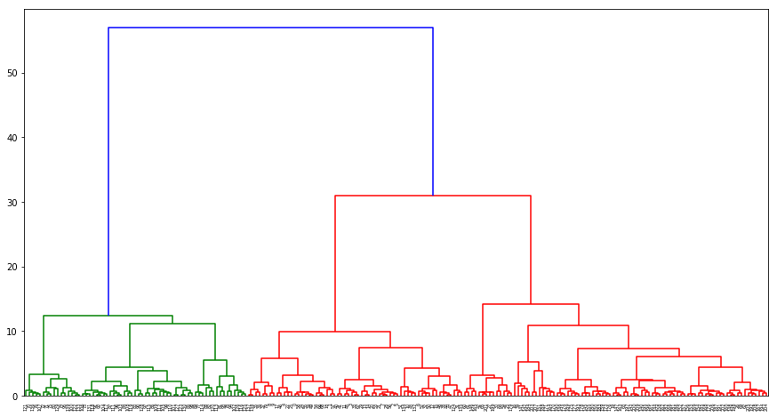
In the hierarchical clustering binary tree, the \(x\)-axis represents the original categories of the data points, which are the sample numbers, while the \(y\)-axis represents the distances between the categories.
Specifically, the height at which the horizontal line in the figure lies indicates the distance at which the categories are merged. If the distance between two adjacent horizontal lines is larger, it means that the distance at which the previous categories are merged is farther, which also indicates that they may not belong to the same category and do not need to be merged.
In the above figure, the \(y\)-difference corresponding to the blue line is the largest, which indicates that the red and green branches are very likely not to belong to the same category.
29.5. Pruning the Hierarchical Clustering Binary Tree#
Above, we used
dendrogram()
to plot the binary tree. You will find that as the number of
samples increases, the leaf nodes become denser, ultimately
resulting in a reduced visibility for identifying different
categories through the binary tree.
In fact, you can specify multiple parameters to prune the complete binary tree result to make it more visually appealing.
{exercise-start}
:label: chapter03_05_3
Challenge: Prune the hierarchical clustering binary tree of wheat seeds.
Hint: Modify the parameters
truncate_mode,
p,
show_leaf_counts,
show_contracted.
{exercise-end}
plt.figure(figsize=(15, 8))
## 代码开始 ### (≈ 1 行代码)

## 代码结束 ###
plt.show()
{solution-start} chapter03_05_3
:class: dropdown
plt.figure(figsize=(15, 8))
### Code starts ### (≈ 1 line of code)
hierarchy.dendrogram(Z, truncate_mode='lastp', p=15, show_leaf_counts=True, show_contracted=True)
### Code ends ###
plt.show()
{solution-end}
Expected output
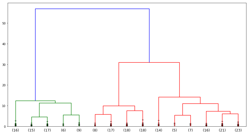
The binary tree looks more aesthetically pleasing at this time. So, how many categories are the wheat seeds roughly determined to be in this challenge? The following gives a suggestion through the hierarchical clustering binary tree:
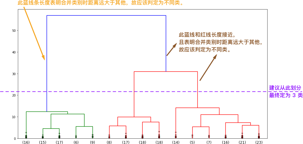
Therefore, it is finally recommended to divide the wheat seed dataset into 3 categories, that is, it contains 3 different varieties of wheat grains.