
60. Convolutional Neural Network Construction#
60.1. Introduction#
Previously, we have learned the principles of convolutional neural networks, especially elaborating on key components such as convolutional layers and pooling layers. This experiment will focus on how to build a convolutional neural network using a deep learning framework and complete model training.
60.2. Key Points#
Construction with TensorFlow High-Level APIs
Construction with TensorFlow Low-Level APIs
Construction with PyTorch Low-Level APIs
Construction with PyTorch High-Level APIs
In the previous experiments, we have learned how to build and train artificial neural networks using TensorFlow and PyTorch. In fact, the process of building a convolutional neural network is no different from that of a fully connected neural network, except that special components required for a convolutional neural network are added to the neural network.
Next, the experiment will attempt to build a convolutional
neural network using the four methods learned previously,
namely: the low-level
tf.nn
module and the high-level
tf.keras
module of TensorFlow, as well as the
nn.Module
and
nn.Sequential
modules of PyTorch.
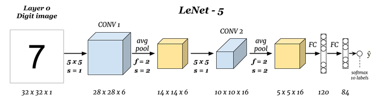
The experiment still uses the familiar MNIST dataset. This dataset has a moderate number of samples and is very suitable for practice. For the neural network, the classic LeNet-5 convolutional neural network structure invented by Yann LeCun in 1998 is selected.
60.3. Data Preprocessing#
For the MNIST dataset, we have already loaded it using TensorFlow and PyTorch respectively. In fact, the API of the deep learning framework to load the dataset directly downloads the corresponding dataset from LeCun’s website. Here, we download the mirror file.
# 直接运行下载数据文件
wget -nc "https://cdn.aibydoing.com/aibydoing/files/MNIST_data.zip"
unzip -o "MNIST_data.zip"
文件 “MNIST_data.zip” 已经存在;不获取。

Archive:  MNIST_data.zip
 extracting: MNIST_data/t10k-labels-idx1-ubyte.gz
 extracting: MNIST_data/train-labels-idx1-ubyte.gz
  inflating: MNIST_data/t10k-images-idx3-ubyte.gz
  inflating: MNIST_data/train-images-idx3-ubyte.gz
The dataset contains a total of four files, namely:
-
Training samples:
train-images-idx3-ubyte.gz -
Training labels:
train-labels-idx1-ubyte.gz -
Test samples:
t10k-images-idx3-ubyte.gz -
Test labels:
t10k-labels-idx1-ubyte.gz
The data is stored in the IDX file format and needs to be read out first.
# 此段数据读取代码无需掌握
import gzip
import numpy as np


def read_mnist(images_path, labels_path):
    with gzip.open("MNIST_data/" + labels_path, "rb") as labelsFile:
        y = np.frombuffer(labelsFile.read(), dtype=np.uint8, offset=8)

    with gzip.open("MNIST_data/" + images_path, "rb") as imagesFile:
        X = (
            np.frombuffer(imagesFile.read(), dtype=np.uint8, offset=16)
            .reshape(len(y), 784)
            .reshape(len(y), 28, 28, 1)
        )

    return X, y


train = {}
test = {}

train["X"], train["y"] = read_mnist(
    "train-images-idx3-ubyte.gz", "train-labels-idx1-ubyte.gz"
)
test["X"], test["y"] = read_mnist(
    "t10k-images-idx3-ubyte.gz", "t10k-labels-idx1-ubyte.gz"
)

train["X"].shape, train["y"].shape, test["X"].shape, test["y"].shape
((60000, 28, 28, 1), (60000,), (10000, 28, 28, 1), (10000,))
As can be seen, the training set contains 60,000 images of size \(28 \times 28\), and for grayscale images, the color channel is retained as 1. The test set contains 10,000 samples. We can visualize the first sample.
from matplotlib import pyplot as plt

%matplotlib inline

plt.imshow(train["X"][0].reshape(28, 28), cmap=plt.cm.gray_r)
<matplotlib.image.AxesImage at 0x13e380100>

Return to the above schematic diagram of the LeNet-5 network
structure. You will see that the input image size of the
original LeNet-5 structure is
32x32x1. Therefore, our data preprocessing here is not yet
complete. We can achieve the effect by padding 2 zeros on
each outer circle of the
28x28x1
image, so that we can implement the LeNet-5 convolutional
neural network exactly.

Meanwhile, since the final output of LeNet-5 is Softmax, we need to perform one-hot encoding on the labels, which we have learned in the previous experiments.
# 样本 padding 填充
X_train = np.pad(train["X"], ((0, 0), (2, 2), (2, 2), (0, 0)), "constant")
X_test = np.pad(test["X"], ((0, 0), (2, 2), (2, 2), (0, 0)), "constant")
# 标签独热编码
y_train = np.eye(10)[train["y"].reshape(-1)]
y_test = np.eye(10)[test["y"].reshape(-1)]

X_train.shape, X_test.shape, y_train.shape, y_test.shape
((60000, 32, 32, 1), (10000, 32, 32, 1), (60000, 10), (10000, 10))
We can confirm the modification by visualization again.
from matplotlib import pyplot as plt

%matplotlib inline

plt.imshow(X_train[0].reshape(32, 32), cmap=plt.cm.gray_r)
<matplotlib.image.AxesImage at 0x13e44a0e0>

60.4. High-Level
tf.keras
Construction in TensorFlow#
Since the high-level API is easier to use, we first use Keras provided by TensorFlow to build the LeNet-5 convolutional neural network. Before that, it is necessary to understand the convolutional layer and pooling layer to be used.
Among them, the convolutional layer classes included under
tf.keras.layers
🔗
are:
-
tf.keras.layers.Conv1D🔗: Generally used for one-dimensional convolution on text or time series. -
tf.keras.layers.Conv2D🔗: Generally used for two-dimensional convolution in the image space. -
tf.keras.layers.Conv3D🔗. Generally used for three-dimensional convolution in processing videos and other multi-frame images.
For the detailed differences among the three, you can read
Intuitive understanding…. In fact, we generally only use
tf.keras.layers.Conv2D
in image processing.
The convolutional layer class contains many parameters, but generally what we use are nothing more than:
-
filters: The number of convolutional kernels, an integer. -
kernel_size: The size of the convolutional kernel, a tuple. -
strides: The convolutional stride, a tuple. -
padding:"valid"or"same".
Pay special attention that if the convolutional layer is the
first layer in the model, the
input_shape
parameter needs to be provided. For example,
input_shape=(128,
                      128,
                      3)
represents a 128x128 RGB image. At this time, a default
parameter
data_format="channels_last"
will be associated, that is, the number of color channels 3
is at the end. Of course, if your
input_shape=(3,
                      128,
                      128)
, you need to specify the parameter
data_format="channels_first".
Secondly, it should be noted that
padding
supports two parameters, namely
"valid"
or
"same"
(case-sensitive). Now let’s talk about the meanings of these
two parameters in TensorFlow. Suppose a row of the input
matrix is as follows, containing 13 units.

When the parameter is
"valid"
(default), the pixels that cannot be convolved will be
discarded. That is, no padding is performed on the margins,
which is equivalent to not requiring a Padding operation.

When the parameter is
"same", padding with
0
is performed to ensure that every input pixel can be
convolved.

As shown above, three grids with a value of
0
are added to ensure that every input pixel can be convolved.
When adding, in the case of an odd number as above, by
default, there will be more on the right side.
In addition, when processing images, the pooling layer
generally only uses classes with 2D, such as the average
pooling
tf.keras.layers.AveragePooling2D
required in the LeNet-5 network
🔗.
Two commonly used parameters in the pooling layer:
pool_size
and
stride. The default value of the pooling window for
pool_size
is
(2,
                      2)
, which means reducing the tensor to half of its original
size.
stride
represents the factor for reducing the scale. For example,
2
will halve the input tensor. If it is
None, the default value is
pool_size.
Next, we use the high-level Keras API provided by TensorFlow to build the LeNet-5 convolutional neural network. Except for the known parameters shown in the figure, other parameters such as the number of convolutional kernels and activation functions are specified according to the data provided in the original paper.
import tensorflow as tf

model = tf.keras.Sequential()  # 构建顺序模型

# 卷积层,6 个 5x5 卷积核,步长为 1,relu 激活,第一层需指定 input_shape
model.add(
    tf.keras.layers.Conv2D(
        filters=6,
        kernel_size=(5, 5),
        strides=(1, 1),
        activation="relu",
        input_shape=(32, 32, 1),
    )
)
# 平均池化,池化窗口默认为 2
model.add(tf.keras.layers.AveragePooling2D(pool_size=(2, 2), strides=2))
# 卷积层,16 个 5x5 卷积核,步为 1,relu 激活
model.add(
    tf.keras.layers.Conv2D(
        filters=16, kernel_size=(5, 5), strides=(1, 1), activation="relu"
    )
)
# 平均池化,池化窗口默认为 2
model.add(tf.keras.layers.AveragePooling2D(pool_size=(2, 2), strides=2))
# 需展平后才能与全连接层相连
model.add(tf.keras.layers.Flatten())
# 全连接层,输出为 120,relu 激活
model.add(tf.keras.layers.Dense(units=120, activation="relu"))
# 全连接层,输出为 84,relu 激活
model.add(tf.keras.layers.Dense(units=84, activation="relu"))
# 全连接层,输出为 10,Softmax 激活
model.add(tf.keras.layers.Dense(units=10, activation="softmax"))
# 查看网络结构
model.summary()
Model: "sequential"
_________________________________________________________________
 Layer (type)                Output Shape              Param #
=================================================================
 conv2d (Conv2D)             (None, 28, 28, 6)         156

 average_pooling2d (Average  (None, 14, 14, 6)         0
 Pooling2D)

 conv2d_1 (Conv2D)           (None, 10, 10, 16)        2416

 average_pooling2d_1 (Avera  (None, 5, 5, 16)          0
 gePooling2D)

 flatten (Flatten)           (None, 400)               0

 dense (Dense)               (None, 120)               48120

 dense_1 (Dense)             (None, 84)                10164

 dense_2 (Dense)             (None, 10)                850

=================================================================
Total params: 61706 (241.04 KB)
Trainable params: 61706 (241.04 KB)
Non-trainable params: 0 (0.00 Byte)
_________________________________________________________________
As you can see, the network structure is exactly the same as that shown in the figure. Next, we can compile the model and complete the training and evaluation.
# 编译模型,Adam 优化器,多分类交叉熵损失函数,准确度评估
model.compile(optimizer="adam", loss="categorical_crossentropy", metrics=["accuracy"])
# 模型训练及评估
model.fit(X_train, y_train, batch_size=64, epochs=2, validation_data=(X_test, y_test))
Epoch 1/2
938/938 [==============================] - 6s 7ms/step - loss: 0.3219 - accuracy: 0.9330 - val_loss: 0.0781 - val_accuracy: 0.9752
Epoch 2/2
938/938 [==============================] - 6s 6ms/step - loss: 0.0668 - accuracy: 0.9796 - val_loss: 0.0607 - val_accuracy: 0.9813
<keras.src.callbacks.History at 0x290564c10>
60.5. Construction with
Low-Level
tf.nn
in TensorFlow#
The low-level API of TensorFlow mainly uses the
tf.nn
module. After constructing the forward computation graph, a
session is established to complete the model training. Among
them, the convolution function is
tf.nn.conv2d
🔗, and the average pooling function is
tf.nn.avg_pool
🔗. It is worth noting that although the meanings of most
parameters are similar to those in Keras, their usage is
different. You need to learn according to the following
example code and the official documentation.
When we implement using
tf.nn, we need to initialize the weights (convolution kernels)
ourselves just like in the previous fully connected neural
network. Here, we can use
random_normal
to randomly generate weight values according to any given
matrix size.
class Model(object):
    def __init__(self):
        # 随机初始化张量参数
        self.conv_W1 = tf.Variable(tf.random.normal(shape=(5, 5, 1, 6)))
        self.conv_W2 = tf.Variable(tf.random.normal(shape=(5, 5, 6, 16)))
        self.fc_W1 = tf.Variable(tf.random.normal(shape=(5 * 5 * 16, 120)))
        self.fc_W2 = tf.Variable(tf.random.normal(shape=(120, 84)))
        self.out_W = tf.Variable(tf.random.normal(shape=(84, 10)))

        self.fc_b1 = tf.Variable(tf.zeros(120))
        self.fc_b2 = tf.Variable(tf.zeros(84))
        self.out_b = tf.Variable(tf.zeros(10))

    def __call__(self, x):
        x = tf.cast(x, tf.float32)  # 转换输入数据类型
        # 卷积层 1: Input = 32x32x1. Output = 28x28x6.
        conv1 = tf.nn.conv2d(x, self.conv_W1, strides=[1, 1, 1, 1], padding="VALID")
        # RELU 激活
        conv1 = tf.nn.relu(conv1)
        # 池化层 1: Input = 28x28x6. Output = 14x14x6.
        pool1 = tf.nn.avg_pool(
            conv1, ksize=[1, 2, 2, 1], strides=[1, 2, 2, 1], padding="VALID"
        )
        # 卷积层 2: Input = 14x14x6. Output = 10x10x16.
        conv2 = tf.nn.conv2d(pool1, self.conv_W2, strides=[1, 1, 1, 1], padding="VALID")
        # RELU 激活
        conv2 = tf.nn.relu(conv2)
        # 池化层 2: Input = 10x10x16. Output = 5x5x16.
        pool2 = tf.nn.avg_pool(
            conv2, ksize=[1, 2, 2, 1], strides=[1, 2, 2, 1], padding="VALID"
        )
        # 展平. Input = 5x5x16. Output = 400.
        flatten = tf.reshape(pool2, [-1, 5 * 5 * 16])
        # 全连接层
        fc1 = tf.nn.relu(tf.add(tf.matmul(flatten, self.fc_W1), self.fc_b1))
        fc2 = tf.nn.relu(tf.add(tf.matmul(fc1, self.fc_W2), self.fc_b2))
        outs = tf.add(tf.matmul(fc2, self.out_W), self.out_b)
        return outs
The following process is very similar to the previous one of using TensorFlow to complete DIGITS classification. Define the loss function and the accuracy calculation function respectively.
def loss_fn(model, x, y):
    preds = model(x)
    return tf.reduce_mean(
        tf.nn.softmax_cross_entropy_with_logits(logits=preds, labels=y)
    )
def accuracy_fn(logits, labels):
    preds = tf.argmax(logits, axis=1)  # 取值最大的索引,正好对应字符标签
    labels = tf.argmax(labels, axis=1)
    return tf.reduce_mean(tf.cast(tf.equal(preds, labels), tf.float32))
If we use the low-level API of TensorFlow to build a neural network, we need to implement the mini-batch training process ourselves to prevent the memory from exploding due to too much data being passed in at once. Similarly, this part of the code has been implemented in the previous experiments, so we can directly take it over and modify the appropriate number of iterations and mini-batch size.
from sklearn.model_selection import KFold
from tqdm.notebook import tqdm

EPOCHS = 2  # 迭代此时
BATCH_SIZE = 64  # 每次迭代的批量大小
LEARNING_RATE = 0.001  # 学习率

model = Model()  # 实例化模型类

for epoch in range(EPOCHS):  # 设定全数据集迭代次数
    indices = np.arange(len(X_train))  # 生成训练数据长度规则序列
    np.random.shuffle(indices)  # 对索引序列进行打乱,保证为随机数据划分
    batch_num = int(len(X_train) / BATCH_SIZE)  # 根据批量大小求得要划分的 batch 数量
    kf = KFold(n_splits=batch_num)  # 将数据分割成 batch 数量份
    # KFold 划分打乱后的索引序列,然后依据序列序列从数据中抽取 batch 样本
    for _, index in tqdm(kf.split(indices), desc="Training"):
        X_batch = X_train[indices[index]]  # 按打乱后的序列取出数据
        y_batch = y_train[indices[index]]

        with tf.GradientTape() as tape:  # 追踪梯度
            loss = loss_fn(model, X_batch, y_batch)

        trainable_variables = [
            model.conv_W1,
            model.conv_W2,
            model.fc_W1,
            model.fc_W2,
            model.out_W,
            model.fc_b1,
            model.fc_b2,
            model.out_b,
        ]  # 需优化参数列表
        grads = tape.gradient(loss, trainable_variables)  # 计算梯度

        optimizer = tf.optimizers.Adam(learning_rate=LEARNING_RATE)  # Adam 优化器
        optimizer.apply_gradients(zip(grads, trainable_variables))  # 更新梯度

    # 每一次 Epoch 执行小批量测试,防止内存不足
    indices_test = np.arange(len(X_test))
    batch_num_test = int(len(X_test) / BATCH_SIZE)
    kf_test = KFold(n_splits=batch_num_test)
    test_acc = 0
    for _, index in tqdm(kf_test.split(indices_test), desc="Testing"):
        X_test_batch = X_test[indices_test[index]]
        y_test_batch = y_test[indices_test[index]]
        batch_acc = accuracy_fn(model(X_test_batch), y_test_batch)  # 计算准确度
        test_acc += batch_acc  # batch 准确度求和

    accuracy = test_acc / batch_num_test  # 测试集准确度
    print(f"Epoch [{epoch+1}/{EPOCHS}], Accuracy: [{accuracy:.2f}], Loss: [{loss:.4f}]")
Epoch [1/2], Accuracy: [0.89], Loss: [25219.9238]
Epoch [2/2], Accuracy: [0.91], Loss: [12266.0176]
You may find that the same network structure yields better results when using Keras. In fact, this is the advantage of using the high-level API, which has been fully optimized in details such as learning rate and weight initialization. Therefore, generally speaking, for networks that can be built using the high-level API of TensorFlow, we will not use the low-level API to cause trouble for ourselves. However, the low-level API is more flexible and can meet the needs of advanced developers or academic researchers.
60.6. Building with
Low-Level
nn.Module
in PyTorch#
We have used two common processes provided by TensorFlow to build the LeNet-5 convolutional neural network for MNIST training. Next, we will use the APIs provided by PyTorch to reconstruct the entire process of LeNet-5.
First, we build a neural network based on
nn.Module. Remember? Here, we need to inherit from the base class
nn.Module
to implement a custom neural network structure.
import torch
import torch.nn as nn
import torch.nn.functional as F


class LeNet(nn.Module):
    def __init__(self):
        super(LeNet, self).__init__()
        # 卷积层 1
        self.conv1 = nn.Conv2d(
            in_channels=1, out_channels=6, kernel_size=(5, 5), stride=1
        )
        # 池化层 1
        self.pool1 = nn.AvgPool2d(kernel_size=(2, 2))
        # 卷积层 2
        self.conv2 = nn.Conv2d(
            in_channels=6, out_channels=16, kernel_size=(5, 5), stride=1
        )
        # 池化层 2
        self.pool2 = nn.AvgPool2d(kernel_size=(2, 2))
        # 全连接层
        self.fc1 = nn.Linear(in_features=5 * 5 * 16, out_features=120)
        self.fc2 = nn.Linear(in_features=120, out_features=84)
        self.fc3 = nn.Linear(in_features=84, out_features=10)

    def forward(self, x):
        x = F.relu(self.conv1(x))
        x = self.pool1(x)
        x = F.relu(self.conv2(x))
        x = self.pool2(x)
        x = x.reshape(-1, 5 * 5 * 16)
        x = F.relu(self.fc1(x))
        x = F.relu(self.fc2(x))
        x = F.softmax(self.fc3(x), dim=1)
        return x
It is worth noting that the parameters of the convolutional
layer in PyTorch are different from those in TensorFlow.
PyTorch does not have a parameter for the number of
convolutional kernels in TensorFlow. Instead, we need to set
out_channels
to represent the number of convolutional kernels. This is
actually easy to understand. An image with
in_channels
channels is output through
out_channels
channels, which is naturally processed by
out_channels
convolutional kernels.
The pooling layer and the fully connected layer should be
easy to understand. In particular, there is no class related
to the Flatten layer in PyTorch. Therefore, we use
x.reshape(-1,
                      5*5*16)
in the network to convert the tensor into the shape we need.
Next, instantiate the custom model class and print out the model structure.
model = LeNet()
model
LeNet(
  (conv1): Conv2d(1, 6, kernel_size=(5, 5), stride=(1, 1))
  (pool1): AvgPool2d(kernel_size=(2, 2), stride=(2, 2), padding=0)
  (conv2): Conv2d(6, 16, kernel_size=(5, 5), stride=(1, 1))
  (pool2): AvgPool2d(kernel_size=(2, 2), stride=(2, 2), padding=0)
  (fc1): Linear(in_features=400, out_features=120, bias=True)
  (fc2): Linear(in_features=120, out_features=84, bias=True)
  (fc3): Linear(in_features=84, out_features=10, bias=True)
)
Unfortunately, PyTorch cannot print out the changes in tensor dimensions between models like TensorFlow can. However, you can use third-party tools such as Model summary in PyTorch to achieve this. We will not attempt it in the experiment.
Next, we test the model by inputting a sample tensor to see
if it can perform calculations normally between the custom
models and whether the output shape meets expectations. When
we take out the first sample
X_train[0], its shape is
(32,
                      32,
                      1)
. This does not conform to the shape of the sample input in
PyTorch. We need to convert the sample into a shape that the
network can accept according to the characteristics of
PyTorch.
model(torch.Tensor(X_train[0]).reshape(-1, 1, 32, 32))
tensor([[0.0959, 0.0295, 0.1106, 0.0372, 0.0689, 0.1577, 0.2842, 0.0583, 0.0939,
         0.0638]], grad_fn=<SoftmaxBackward0>)
In the above example,
X_train[0]
is first converted from a NumPy array to a PyTorch tensor
and then reshaped to
(-1,
                      1, 32,
                      32)
. Here,
-1
is used to adapt to the number of multiple samples later,
which is also consistent with the previous scenarios where
we used
-1. The
1
represents one channel, which corresponds to the
in_channels
of the network’s convolutional layer, and the subsequent
32
is, of course, the size of the sample tensor.
Finally, the output for a single sample is
torch.Size([1,
                      10])
, which is also consistent with the expected output size of
Softmax.
Now that we have the network structure, the next step is
naturally to define the dataset and start training. Remember
the
DataLoader
in PyTorch introduced earlier? It allows us to easily read
mini-batch data. Now, we can also convert the custom NumPy
array into a
DataLoader
loader.
Creating a custom
DataLoader
data loader is divided into two steps. First, use
torch.utils.data.TensorDataset(images,
                      labels)
🔗
to convert the PyTorch tensors into a dataset.
import torch.utils.data

# 依次传入样本和标签张量,制作训练数据集和测试数据集
train_data = torch.utils.data.TensorDataset(
    torch.Tensor(X_train), torch.Tensor(train["y"])
)
test_data = torch.utils.data.TensorDataset(
    torch.Tensor(X_test), torch.Tensor(test["y"])
)

train_data, test_data
(<torch.utils.data.dataset.TensorDataset at 0x294c46e90>,
 <torch.utils.data.dataset.TensorDataset at 0x294c473d0>)
In the above code, the samples are passed the PyTorch
tensors converted from
X_train
and
X_test. The labels are passed
train['y']
and
test['y']
before one-hot encoding, rather than the one-hot encoded
y_train
or
y_test
used in TensorFlow above. The reason is that PyTorch’s loss
functions do not require the labels to be in one-hot encoded
form and can handle the original numerical labels.
Then, we use the
DataLoader
data loader to load the dataset, setting the
batch_size. Generally, the training data is shuffled, while the test
data does not need to be shuffled.
train_loader = torch.utils.data.DataLoader(train_data, batch_size=64, shuffle=True)
test_loader = torch.utils.data.DataLoader(test_data, batch_size=64, shuffle=False)

train_loader, test_loader
(<torch.utils.data.dataloader.DataLoader at 0x174ea6ec0>,
 <torch.utils.data.dataloader.DataLoader at 0x174ea66e0>)
Define the cross-entropy loss function and the Adam optimizer. The following process is very similar to the previous PyTorch neural network construction experiment.
loss_fn = nn.CrossEntropyLoss()  # 交叉熵损失函数
opt = torch.optim.Adam(model.parameters(), lr=0.001)  # Adam 优化器
Finally, define the training function. Here, directly use
the previous code, just note that
images
needs to be
reshaped into the shape of
(-1,
                      1, 32,
                      32)
. And
labels
needs to be converted to the
torch.LongTensor
type to prevent errors.
def fit(epochs, model, opt):
    # 全数据集迭代 epochs 次
    print("================ Start Training =================")
    for epoch in range(epochs):
        # 从数据加载器中读取 Batch 数据开始训练
        for i, (images, labels) in enumerate(train_loader):
            images = images.reshape(-1, 1, 32, 32)  # 对特征数据展平,变成 784
            labels = labels.type(torch.LongTensor)  # 真实标签

            outputs = model(images)  # 前向传播
            loss = loss_fn(outputs, labels)  # 传入模型输出和真实标签

            opt.zero_grad()  # 优化器梯度清零,否则会累计
            loss.backward()  # 从最后 loss 开始反向传播
            opt.step()  # 优化器迭代

            # 自定义训练输出样式
            if (i + 1) % 100 == 0:
                print(
                    "Epoch [{}/{}], Batch [{}/{}], Train loss: [{:.3f}]".format(
                        epoch + 1, epochs, i + 1, len(train_loader), loss.item()
                    )
                )

        # 每个 Epoch 执行一次测试
        correct = 0
        total = 0
        for images, labels in test_loader:
            images = images.reshape(-1, 1, 32, 32)
            labels = labels.type(torch.LongTensor)

            outputs = model(images)
            # 得到输出最大值 _ 及其索引 predicted
            _, predicted = torch.max(outputs.data, 1)

            correct += (predicted == labels).sum().item()  # 如果预测结果和真实值相等则计数 +1
            total += labels.size(0)  # 总测试样本数据计数

        print(
            "============= Test accuracy: {:.3f} ==============".format(correct / total)
        )
Now you can start training:
fit(epochs=2, model=model, opt=opt)
================ Start Training =================
Epoch [1/2], Batch [100/938], Train loss: [1.667]
Epoch [1/2], Batch [200/938], Train loss: [1.596]
Epoch [1/2], Batch [300/938], Train loss: [1.703]
Epoch [1/2], Batch [400/938], Train loss: [1.596]
Epoch [1/2], Batch [500/938], Train loss: [1.504]
Epoch [1/2], Batch [600/938], Train loss: [1.526]
Epoch [1/2], Batch [700/938], Train loss: [1.519]
Epoch [1/2], Batch [800/938], Train loss: [1.499]
Epoch [1/2], Batch [900/938], Train loss: [1.489]
============= Test accuracy: 0.969 ==============
Epoch [2/2], Batch [100/938], Train loss: [1.491]
Epoch [2/2], Batch [200/938], Train loss: [1.477]
Epoch [2/2], Batch [300/938], Train loss: [1.494]
Epoch [2/2], Batch [400/938], Train loss: [1.496]
Epoch [2/2], Batch [500/938], Train loss: [1.494]
Epoch [2/2], Batch [600/938], Train loss: [1.462]
Epoch [2/2], Batch [700/938], Train loss: [1.476]
Epoch [2/2], Batch [800/938], Train loss: [1.494]
Epoch [2/2], Batch [900/938], Train loss: [1.475]
============= Test accuracy: 0.973 ==============
60.7. PyTorch Advanced
nn.Sequential
Construction#
In PyTorch, networks constructed using
nn.Module
can generally be refactored using
nn.Sequential. Since there is no Flatten class in PyTorch, a Flatten
needs to be implemented first before the conversion can be
completed.
class Flatten(nn.Module):
    def forward(self, input):
        return input.reshape(input.size(0), -1)


# 构建 Sequential 容器结构
model_s = nn.Sequential(
    nn.Conv2d(1, 6, (5, 5), 1),
    nn.ReLU(),
    nn.AvgPool2d((2, 2)),
    nn.Conv2d(6, 16, (5, 5), 1),
    nn.ReLU(),
    nn.AvgPool2d((2, 2)),
    Flatten(),
    nn.Linear(5 * 5 * 16, 120),
    nn.ReLU(),
    nn.Linear(120, 84),
    nn.ReLU(),
    nn.Linear(84, 10),
    nn.Softmax(dim=1),
)

model_s
Sequential(
  (0): Conv2d(1, 6, kernel_size=(5, 5), stride=(1, 1))
  (1): ReLU()
  (2): AvgPool2d(kernel_size=(2, 2), stride=(2, 2), padding=0)
  (3): Conv2d(6, 16, kernel_size=(5, 5), stride=(1, 1))
  (4): ReLU()
  (5): AvgPool2d(kernel_size=(2, 2), stride=(2, 2), padding=0)
  (6): Flatten()
  (7): Linear(in_features=400, out_features=120, bias=True)
  (8): ReLU()
  (9): Linear(in_features=120, out_features=84, bias=True)
  (10): ReLU()
  (11): Linear(in_features=84, out_features=10, bias=True)
  (12): Softmax(dim=1)
)
Similar to the previous experiment, we need to rewrite the optimizer code to optimize the new model parameters and start training.
opt_s = torch.optim.Adam(model_s.parameters(), lr=0.001)  # Adam 优化器
fit(epochs=2, model=model_s, opt=opt_s)
================ Start Training =================
Epoch [1/2], Batch [100/938], Train loss: [1.610]
Epoch [1/2], Batch [200/938], Train loss: [1.505]
Epoch [1/2], Batch [300/938], Train loss: [1.556]
Epoch [1/2], Batch [400/938], Train loss: [1.537]
Epoch [1/2], Batch [500/938], Train loss: [1.495]
Epoch [1/2], Batch [600/938], Train loss: [1.525]
Epoch [1/2], Batch [700/938], Train loss: [1.484]
Epoch [1/2], Batch [800/938], Train loss: [1.490]
Epoch [1/2], Batch [900/938], Train loss: [1.488]
============= Test accuracy: 0.968 ==============
Epoch [2/2], Batch [100/938], Train loss: [1.490]
Epoch [2/2], Batch [200/938], Train loss: [1.495]
Epoch [2/2], Batch [300/938], Train loss: [1.492]
Epoch [2/2], Batch [400/938], Train loss: [1.489]
Epoch [2/2], Batch [500/938], Train loss: [1.461]
Epoch [2/2], Batch [600/938], Train loss: [1.477]
Epoch [2/2], Batch [700/938], Train loss: [1.478]
Epoch [2/2], Batch [800/938], Train loss: [1.492]
Epoch [2/2], Batch [900/938], Train loss: [1.476]
============= Test accuracy: 0.977 ==============
60.8. Summary#
In this experiment, we learned how to build the classic LeNet-5 convolutional neural network structure using TensorFlow and PyTorch. Although the structure of LeNet-5 is very simple, it includes all the commonly used components of convolutional neural networks, fully meeting the purpose of the exercise. Everyone must combine the previous explanations and experiments of TensorFlow and PyTorch to understand the four different methods used in this experiment. This is very helpful for understanding and independently building more complex deep neural networks in the future.