Pro Membership

Pro Membership is a membership plan created by the author to maintain and update this tutorial. You can get more benefits and services, click to view details.

41. Practical Applications of Automated Machine Learning#

41.1. Introduction#

auto-sklearn is an automated machine learning framework developed based on scikit-learn. It continues the ease of use of scikit-learn and further introduces methods of automated machine learning to facilitate non-professional developers in building predictive models. In this experiment, we will learn the use of auto-sklearn and discuss the advantages and disadvantages of automated machine learning.

41.2. Key Points#

Introduction to the auto-sklearn framework
Automated classification and regression algorithms
Advantages and disadvantages of automated machine learning

41.3. Introduction to auto-sklearn#

auto-sklearn As its name implies, you should be able to see its correlation with scikit-learn. Indeed, auto-sklearn is an automated machine learning library developed based on scikit-learn. However, auto-sklearn is not maintained by the scikit-learn development team, but by a third-party organization, automl.org. The personnel of this organization are from the Machine Learning Lab of the University of Freiburg in Germany.

The auto-sklearn framework adopts the global optimization idea of Auto-WEKA that we mentioned in the review section. To improve generalization, auto-sklearn constructs an ensemble learning process based on all models during the global optimization test. To accelerate the optimization process, auto-sklearn uses meta-learning to identify similar datasets and apply existing experience. Auto-sklearn contains a total of 15 classification algorithms, 14 feature preprocessing algorithms, and is responsible for data scaling, classification parameter encoding, and missing value handling.

When using auto-sklearn locally, you need to install it according to the official instructions. The steps are slightly different for different systems. You need to execute the following code to complete the installation.

                      {note}
pip install auto-sklearn

The auto-sklearn API is mainly divided into four parts:

Classification: Training methods related to classification problems.
Regression: Training methods related to regression problems.
Metrics: Algorithm evaluation methods.
Extension Interfaces: Extension interfaces.

Next, we will try to understand the four parts of the interface and learn how to use it.

41.4. Classification Algorithms#

Classification is the most common type of problem in machine learning, and most machine learning algorithms focus on solving classification problems. There are many algorithms in scikit-learn that can be used for classification, including: perceptron, artificial neural network, support vector machine, decision tree, etc. For details, you can read the classification algorithm section in the scikit-learn documentation about Supervised learning.

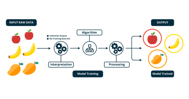
Classification problems can be simply summarized as follows: There are already some data samples and clear classifications for the samples. Now, summarize the patterns from the features of these samples and then use them to determine which category a newly input sample belongs to. For example, the following figure shows a classification process that uses a supervised learning algorithm to distinguish the categories of fruits.

Image description

Source

There is only one classification algorithm API in auto-sklearn, which is AutoSklearnClassifier, and it has a very large number of parameters:

                      autosklearn.classification.AutoSklearnClassifier(time_left_for_this_task=3600, per_run_time_limit=360, initial_configurations_via_metalearning=25, ensemble_size:int=50, ensemble_nbest=50, ensemble_memory_limit=1024, seed=1, ml_memory_limit=3072, include_estimators=None, exclude_estimators=None, include_preprocessors=None, exclude_preprocessors=None, resampling_strategy='holdout', resampling_strategy_arguments=None, tmp_folder=None, output_folder=None, delete_tmp_folder_after_terminate=True, delete_output_folder_after_terminate=True, shared_mode=False, n_jobs: Optional[int] = None, disable_evaluator_output=False, get_smac_object_callback=None, smac_scenario_args=None, logging_config=None, metadata_directory=None)

                    

Next, the important parameters will be introduced in detail:

time_left_for_this_task: The time limit for model search (in seconds). By increasing this value, auto-sklearn has a higher chance of finding a better model, but it takes longer.
per_run_time_limit: The time limit for a single call to the model. If the machine learning algorithm exceeds this time limit, the model fitting will be terminated.
initial_configurations_via_metalearning: Whether the hyperparameter optimization algorithm starts from scratch or uses the metalearning method.
ensemble_size: The number of models selected from the algorithm library to build an ensemble model.
ensemble_memory_limit: The memory limit (in MB) for the overall construction process.
ml_memory_limit: The memory limit (in MB) for a single machine learning algorithm.
include_estimators: A series of alternative algorithm models can be manually specified. If not set, all available algorithms will be used.
include_preprocessors: A series of alternative preprocessing methods can be manually specified. If not set, all available preprocessing methods will be used.
resampling_strategy: The overfitting handling strategy. Cross-validation or holdout can be selected. For holdout, the training and test sets are divided in a 67:33 ratio.
tmp_folder: The output directory for configuration and log files.
output_folder: The output directory for the prediction results of test data.

Next, we will try to use auto-sklearn to complete an example of classification modeling. Here we choose the DIGITS handwritten character example dataset provided by scikit-learn. First, we import this dataset:

                          import numpy as np
from sklearn.datasets import load_digits

digits = load_digits()  # 加载数据集

digits.data.shape, np.unique(digits.target)

It can be seen that the dataset contains a total of 1,797 entries, with 64 features, and there are 10 categories in the target values, which are the digits 0 to 9 respectively.

If we follow the standard scikit-learn modeling process. First, we try to split the data into a 70% training set and a 30% test set. In machine learning, we are used to using such a ratio to split the training set and the test set.

Source

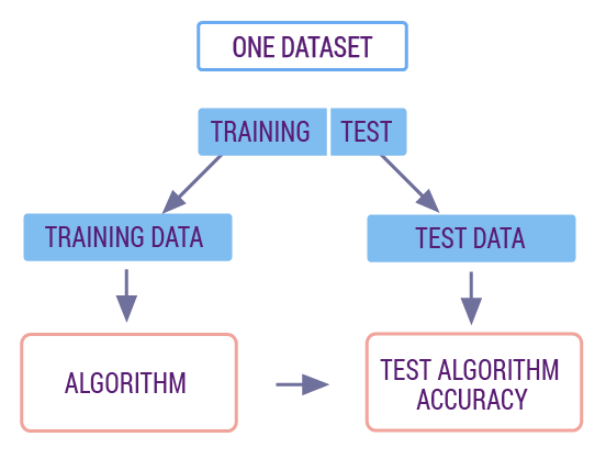
Among them, the training set is used to train the model, while the test set is used to evaluate the quality of the model. The data in the test set will not appear in the training data, which is similar to using new data to make predictions and evaluations on the trained model to ensure the authenticity and reliability of the model quality.

                          from sklearn.model_selection import train_test_split

X_train, X_test, y_train, y_test = train_test_split(
    digits.data, digits.target, test_size=0.3, random_state=42
)  # 切分数据集

X_train.shape, X_test.shape, y_train.shape, y_test.shape

After splitting the training set and the test set, we can start making predictions. When using scikit-learn to solve a machine learning-related problem, our code is mostly the same and mainly consists of several parts:

Call a machine learning method to build the corresponding model model and set the model parameters.
Use the model.fit() method provided by the machine learning model to train the model.
Use the model.predict() method provided by the machine learning model for prediction.

Next, first import the decision tree classifier from scikit-learn. Then use the .fit method to train the model and use .score to get the accuracy of the model on the test set.

                          from sklearn.tree import DecisionTreeClassifier

model = DecisionTreeClassifier()
model.fit(X_train, y_train)  # 训练

model.score(X_test, y_test)  # 评估

Without accident, the accuracy rate of the test set obtained here is approximately around 85%. The above is an integrated machine learning modeling process of scikit-learn.

Next, we try to use auto-sklearn to classify this dataset. In fact, the usage process of auto-sklearn, including the names of the APIs, is basically the same as that of scikit-learn. For the classification algorithms supported by auto-sklearn and their abbreviations, you can check through the official code repository.

We define the model. To improve the search speed, the maximum search time for this task is restricted here. Since there are many warnings during the training process of auto-sklearn, we choose to ignore them.

                          import warnings
from autosklearn.classification import AutoSklearnClassifier

warnings.filterwarnings("ignore")  # 忽略代码警告

# 限制算法搜索最大时间，更快得到结果
auto_model = AutoSklearnClassifier(time_left_for_this_task=120, per_run_time_limit=10)

auto_model

Then, use the .fit method to train the model.

                          auto_model.fit(X_train, y_train)  # 训练 2 分钟
auto_model.score(X_test, y_test)  # 评估

Normally, the results obtained here should be better than those of the decision tree modeling and training using scikit-learn above. If the effect is not ideal, you can further increase the optimization time of the model to facilitate the search for better model parameters.

If you have the condition to practice offline, you can try to train with the default parameters of AutoSklearnClassifier, that is, build models on all algorithms and all preprocessing methods. Normally, you can get an accuracy result of about 99% on the test set. Of course, it takes a very long time to get this result.

There are also some other commonly used methods for the models defined by auto-sklearn. get_models_with_weights can return the model information searched by auto-sklearn:

                          auto_model.get_models_with_weights()

                        

sprint_statistics can return the key statistics of the training process, including the dataset name, the evaluation metrics used, the number of algorithm runs, the evaluation results, etc.

                          auto_model.sprint_statistics()

                        

41.5. Regression Algorithms#

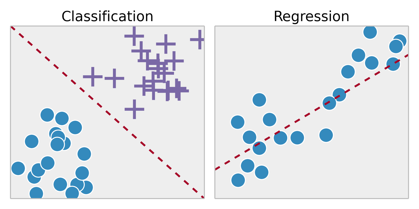
Above, we learned about the methods of auto-sklearn for solving classification problems. In fact, another type of method included in supervised learning (a branch of machine learning) is regression. The biggest difference (feature) between regression problems and classification problems lies in the type of output variable. To elaborate:

For classification problems, the output is a finite number of discrete variables, boolean values, or categorical variables. For example, the handwritten character recognition classification above.
For regression problems, the output is a continuous variable, generally a real number, that is, an exact value. For example, predicting a person’s age.

Source

The linear models included in scikit-learn are least squares regression, perceptron, logistic regression, ridge regression, Bayesian regression, etc., which are imported from the sklearn.linear_model module. The regression algorithms in auto-sklearn are similar to the classification algorithms, and it only contains a core interface AutoSklearnRegressor.

                      autosklearn.regression.AutoSklearnRegressor(time_left_for_this_task=3600, per_run_time_limit=360, initial_configurations_via_metalearning=25, ensemble_size: int = 50, ensemble_nbest=50, ensemble_memory_limit=1024, seed=1, ml_memory_limit=3072, include_estimators=None, exclude_estimators=None, include_preprocessors=None, exclude_preprocessors=None, resampling_strategy='holdout', resampling_strategy_arguments=None, tmp_folder=None, output_folder=None, delete_tmp_folder_after_terminate=True, delete_output_folder_after_terminate=True, shared_mode=False, n_jobs: Optional[int] = None, disable_evaluator_output=False, get_smac_object_callback=None, smac_scenario_args=None, logging_config=None, metadata_directory=None)

                    

Upon careful observation, you will find that the parameter settings of AutoSklearnRegressor are almost exactly the same as those of AutoSklearnClassifier, so we will no longer explain the meanings of the parameters.

In machine learning, some classification methods can actually be used to solve regression problems. Therefore, the search space of AutoSklearnRegressor for regression algorithms is far more than just linear regression and polynomial regression. It also includes algorithms such as K-nearest neighbor regression and decision tree regression. For details, you can check the official code repository.

Next, we will use scikit-learn and auto-sklearn to solve a regression problem. Here, we choose the Boston housing price example dataset.

                          from sklearn.datasets import load_boston

boston = load_boston()  # 加载数据集

boston.data.shape, boston.target.shape

As shown above, the dataset contains 13 features and the target value is the real value of housing prices.

Here, we first choose the linear regression method in scikit-learn to complete the modeling.

                          from sklearn.linear_model import LinearRegression

model = LinearRegression()
model.fit(boston.data, boston.target)

model.score(boston.data, boston.target)

Here, .score returns the coefficient of determination of the regression fit. The coefficient of determination \(R^2\) is used in statistics to measure the proportion of the variation in the dependent variable that can be explained by the independent variable, so as to judge the explanatory power of the statistical model. Simply put, when the value of the coefficient of determination is closer to 1, it means that the relevant equation has a higher reference value. On the contrary, when it is closer to 0, it means that the reference value is lower.

                          from autosklearn.regression import AutoSklearnRegressor

# 限制算法搜索最大时间，更快得到结果
auto_model = AutoSklearnRegressor(time_left_for_this_task=120, per_run_time_limit=10)
auto_model.fit(boston.data, boston.target)

auto_model.score(boston.data, boston.target)

Normally, the \(R^2\) value obtained here should be higher than the result of the above linear regression modeling. If the effect is not ideal, you can further increase the optimization time of the model to search for better model parameters.

Similarly, we can return the key statistical information of the training process.

                          auto_model.sprint_statistics()

                        

41.6. Evaluation Methods#

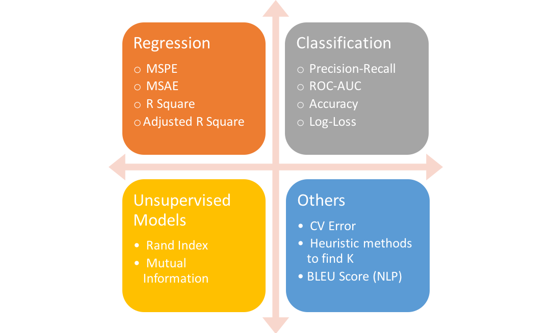
Modeling prediction is the core of machine learning applications, but the evaluation of model quality is essential. Therefore, there are corresponding evaluation methods for algorithm models in machine learning. In the above classification and regression examples, we have already learned two of them. In classification, we often use prediction accuracy for evaluation. For regression models, the evaluation methods include not only \(R^2\), but also mean absolute error, mean squared error, etc.

Source

auto-sklearn basically continues all the model evaluation methods in scikit-learn and places them under autosklearn.metrics. You can also go to the scikit-learn official documentation to learn about the introduction and usage of these methods.

41.7. Advantages and Disadvantages Analysis#

The usage of auto-sklearn is very simple. If you are familiar enough with scikit-learn itself, there are basically no obstacles to learning the use of auto-sklearn. Simply put, when modeling in scikit-learn, you need to import different algorithms from different modules, then set hyperparameters for the algorithms, and even need to use advanced hyperparameter tuning methods such as grid search. However, in auto-sklearn, you only need to import AutoSklearnClassifier or AutoSklearnRegressor. If you have enough time, you don’t even need to set parameters for these two APIs.

But the core problem also emerges, which is time. In the previous examples, in order to obtain results more quickly, the maximum time limit was set for the experiments respectively. If you try it locally without setting a limit, the time taken for auto-sklearn to execute once is extremely long. In particular, this is still on 2 simple example datasets, and the data used in the real environment is often much more complex.

Therefore, through experiments with auto-sklearn, you should be able to further feel the advantages and disadvantages brought by automated machine learning. The advantage lies in its simplicity of use, and you don’t even need to understand the algorithm principle at all. Because it integrates automatic hyperparameter optimization and automatic data processing, it is even much more convenient and faster to use. The disadvantage is that it requires a long search time, dozens of minutes, several hours or even several days.

In addition, automated machine learning is not omnipotent. It may also happen that after spending a lot of time, no ideal model can be found. In this case, if it is handled by machine learning experts, the problems with the data or algorithms may be discovered more quickly.

41.8. Summary#

In this experiment, we learned the use of the auto-sklearn automated machine learning framework. Among them, the methods and steps of applying auto-sklearn to classification and regression problems were mainly introduced, the API parameters were familiarized with, and example exercises were carried out. In addition, the focus of the experiment was to experience the advantages and disadvantages brought by automated machine learning. We must understand this in advance in order to understand how to better utilize machine learning to help ourselves.