52. Building Neural Networks with TensorFlow#
52.1. Introduction#
As a deep learning framework, TensorFlow is of course designed to help us build neural networks more conveniently. Therefore, in this experiment, we will learn how to use TensorFlow to build neural networks and master the important functions and methods for building neural networks with TensorFlow.
52.2. Key Points#
Building Neural Networks with NumPy
Building Neural Networks with TensorFlow
-
Completing DIGITS Classification with TensorFlow
-
Implementing Mini Batch Training with TensorFlow
In the previous experiments, we have understood the working mechanism of TensorFlow and learned to use TensorFlow to participate in calculations. As the most outstanding open-source deep learning framework, TensorFlow has two main advantages in my opinion. The first is the numerical calculation process based on the computational graph, with the ultimate goal of improving the calculation speed. The second is the encapsulation of various commonly used neural network layers to improve the speed of building models.
Therefore, in this experiment, we will learn how to build neural networks using TensorFlow.
52.3. Building Neural Networks with NumPy#
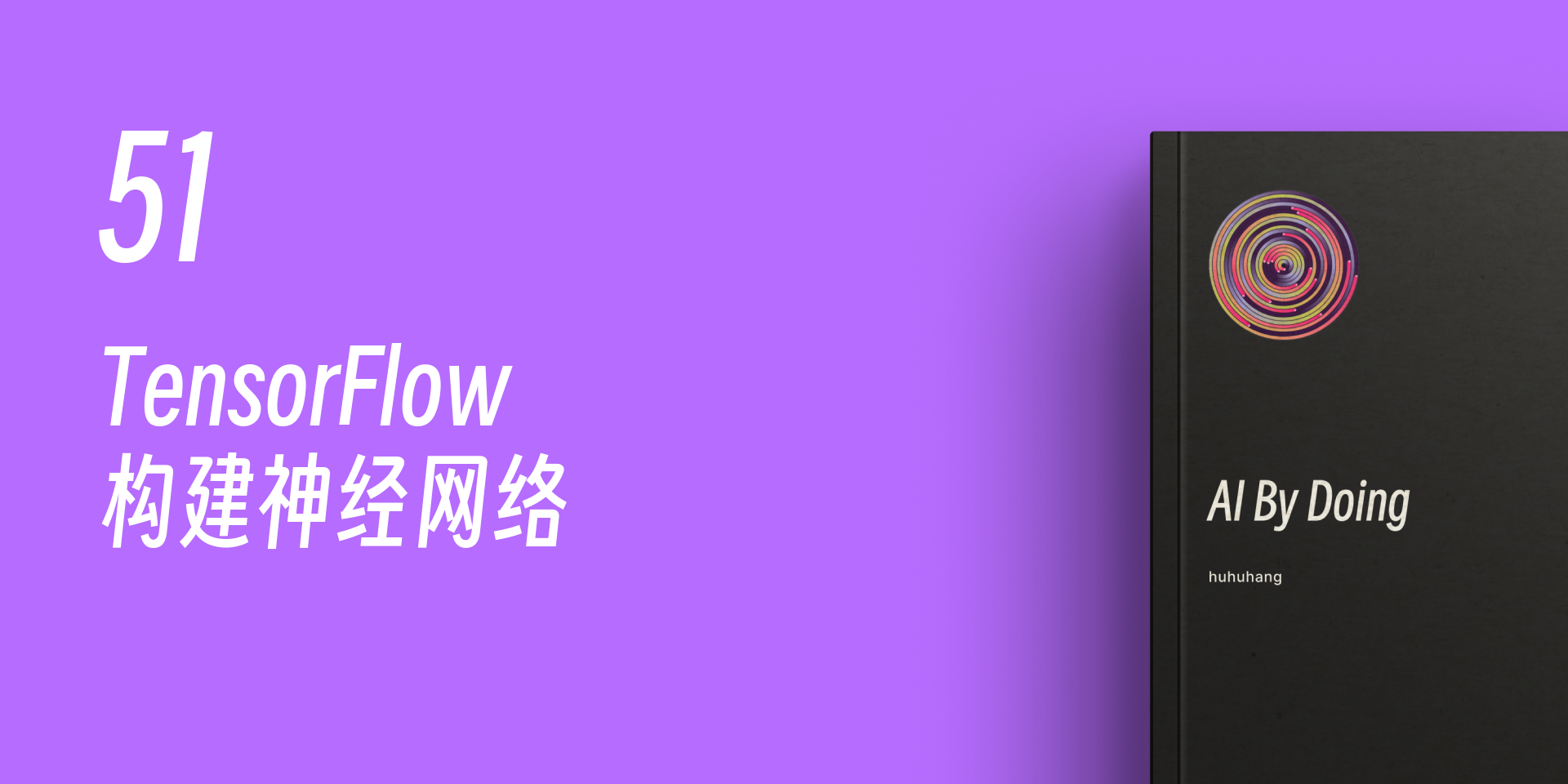
In the experiment of artificial neural networks, we used NumPy to build a simple fully connected neural network. Fully connected means that each of its nodes is connected to every node in the previous layer. For example, the network structure we implemented at that time:
For the implementation of neural networks, it mainly consists of two parts: forward propagation and backward propagation. Forward propagation is of course the calculation from input to output, while backward propagation updates the network weights by calculating gradients. Here, we directly use the code written in the previous perceptron and artificial neural network experiments.
import numpy as np


class NeuralNetwork:
    def __init__(self, X, y, lr):
        """初始化参数"""
        self.input_layer = X
        self.W1 = np.ones((self.input_layer.shape[1], 3))  # 初始化权重全为 1
        self.W2 = np.ones((3, 1))
        self.y = y
        self.lr = lr

    def forward(self):
        """前向传播"""
        self.hidden_layer = sigmoid(np.dot(self.input_layer, self.W1))
        self.output_layer = sigmoid(np.dot(self.hidden_layer, self.W2))
        return self.output_layer

    def backward(self):
        """反向传播"""
        d_W2 = np.dot(
            self.hidden_layer.T,
            (
                2
                * (self.output_layer - self.y)
                * sigmoid_derivative(np.dot(self.hidden_layer, self.W2))
            ),
        )

        d_W1 = np.dot(
            self.input_layer.T,
            (
                np.dot(
                    2
                    * (self.output_layer - self.y)
                    * sigmoid_derivative(np.dot(self.hidden_layer, self.W2)),
                    self.W2.T,
                )
                * sigmoid_derivative(np.dot(self.input_layer, self.W1))
            ),
        )

        # 参数更新
        self.W1 -= self.lr * d_W1
        self.W2 -= self.lr * d_W2
Next, use sample data to complete the neural network training.
wget -nc https://cdn.aibydoing.com/aibydoing/files/course-12-data.csv
import pandas as pd

# 直接运行加载数据集
df = pd.read_csv("course-12-data.csv", header=0)
df.head()  # 预览前 5 行数据
| X0 | X1 | Y | |
|---|---|---|---|
| 0 | 5.1 | 3.5 | -1 |
| 1 | 4.9 | 3.0 | -1 |
| 2 | 4.7 | 3.2 | -1 |
| 3 | 4.6 | 3.1 | -1 |
| 4 | 5.0 | 3.6 | -1 |
from matplotlib import pyplot as plt

%matplotlib inline

X = df[["X0", "X1"]].values  # 输入值
y = df[["Y"]].values  # 真实 y
nn_model = NeuralNetwork(X, y, lr=0.001)  # 定义模型
loss_list = []  # 存放损失数值变化


def sigmoid(x):
    """激活函数"""
    return 1 / (1 + np.exp(-x))


def sigmoid_derivative(x):
    """sigmoid 函数求导"""
    return sigmoid(x) * (1 - sigmoid(x))


# 迭代 200 次
for _ in range(200):
    y_ = nn_model.forward()  # 前向传播
    nn_model.backward()  # 反向传播
    loss = np.square(np.subtract(y, y_)).mean()  # 计算 MSE 损失
    loss_list.append(loss)

plt.plot(loss_list)  # 绘制 loss 曲线变化图
plt.title(f"final loss: {loss}")
Text(0.5, 1.0, 'final loss: 0.8889049031629646')

As can be seen, for a network with only 1 hidden layer, the amount of code implemented using NumPy is already quite a lot. In deep neural networks, there may be hundreds of layers and thousands of neurons, and it is conceivable how complex it would be to implement using NumPy.
52.4. Building Neural Networks with TensorFlow#
If you observe the above code carefully, you will find that as the complexity of the neural network increases, not only does the amount of code keep growing, but the biggest headache lies in solving the gradients. Therefore, the greatest convenience brought by deep learning frameworks such as TensorFlow is that we only need to construct a forward propagation graph of the neural network, and automatic differentiation and parameter update can be achieved during training. Next, we will try to reconstruct the neural network with 1 hidden layer above in the TensorFlow way and finally complete the training.
52.4.1. Processing Tensor Data#
First, we need to complete the conversion of the input data features and target values, and convert them all into tensors.
import tensorflow as tf

tf.get_logger().setLevel("ERROR")

# 将数组转换为常量张量
X = tf.cast(tf.constant(df[["X0", "X1"]].values), tf.float32)
y = tf.constant(df[["Y"]].values)

X.shape, y.shape
(TensorShape([150, 2]), TensorShape([150, 1]))
In the above code,
tf.cast
is mainly used to convert the tensor type to
tf.float32
to unify it with the weight tensor type later. As can be
seen from the output, there are 150 samples, 2 features,
and 1 target value.
52.4.2. Define the Model Class#
Next, we can construct the forward propagation
computational graph. This part is very similar to
constructing the forward propagation process with NumPy,
except that it is replaced with using TensorFlow to
construct. Generally, we will encapsulate the forward
propagation process with a custom model class and randomly
initialize the parameter
\(W\)
using
tf.Variable
provided by TensorFlow.
class Model(object):
    def __init__(self):
        # 初始化权重全为 1,也可以随机初始化
        # 选择变量张量,因为权重后续会不断迭代更新
        self.W1 = tf.Variable(tf.ones([2, 3]))
        self.W2 = tf.Variable(tf.ones([3, 1]))

    def __call__(self, x):
        hidden_layer = tf.nn.sigmoid(tf.linalg.matmul(x, self.W1))  # 隐含层前向传播
        y_ = tf.nn.sigmoid(tf.linalg.matmul(hidden_layer, self.W2))  # 输出层前向传播
        return y_
The above shows the construction method of a standard TensorFlow model class. I hope you can be impressed by it, and this structure will be continuously used in the subsequent construction process of complex neural networks.
We can instantiate the model class and pass in the input array for a simple test.
model = Model()  # 实例化类
y_ = model(X)  # 测试输入
y_.shape  # 输出
TensorShape([150, 1])
Finally, we obtain the predicted output, and its shape should be the same as that of the dataset target values, both being \((150, 1)\).
It is worth noting that in the process of constructing the
network above, we called the
sigmoid
activation function under the
tf.nn
module
🔗.
tf.nn
is a commonly used module in TensorFlow for constructing
neural networks, which contains encapsulated neural
network layers, activation functions, a small number of
loss functions, or other high-level API components.
52.4.3. MSE Loss Function#
Next, we define the loss function required for training.
The loss function is the same as when building with NumPy.
Here, we choose the sum of squares loss function, which is
included in the
tf.losses
module
🔗. This module contains some relatively basic loss
functions, such as the MSE used here.
For more convenient subsequent calls, we need to
encapsulate the calculation method of the
tf.losses.mean_squared_error
MSE loss function into a more complete loss function here.
Specifically, we use the
tf.reduce_mean
method to sum the losses of each sample to obtain the
total loss of the samples.
def loss_fn(model, X, y):
    y_ = model(X)  # 前向传播得到预测值
    # 使用 MSE 损失函数,并使用 reduce_mean 计算样本总损失
    loss = tf.reduce_mean(tf.losses.mean_squared_error(y_true=y, y_pred=y_))
    return loss
Similarly, we can simply test whether the loss function is working properly.
loss = loss_fn(model, X, y)
loss
<tf.Tensor: shape=(), dtype=float32, numpy=1.2723011>
52.4.4. Gradient Descent Optimization Iteration#
After defining the loss function, we can use the gradient
descent method to complete the iterative optimization of
the model parameters. As learned before, Eager Execution
in TensorFlow 2 provides
tf.GradientTape
for tracking gradients, and then we can use the
tape.gradient
method to calculate the gradients.
EPOCHS = 200  # 迭代 200 次
LEARNING_RATE = 0.1  # 学习率

for epoch in range(EPOCHS):
    # 使用 GradientTape 追踪梯度
    with tf.GradientTape() as tape:
        loss = loss_fn(model, X, y)  # 计算 Loss,包含前向传播过程
    # 使用梯度下降法优化迭代
    # 输出模型需优化参数 W1,W2 自动微分结果
    dW1, dW2 = tape.gradient(loss, [model.W1, model.W2])
    model.W1.assign_sub(LEARNING_RATE * dW1)  # 更新梯度
    model.W2.assign_sub(LEARNING_RATE * dW2)

    # 每 100 个 Epoch 输出各项指标
    if epoch == 0:
        print(f"Epoch [000/{EPOCHS}], Loss: [{loss:.4f}]")
    elif (epoch + 1) % 100 == 0:
        print(f"Epoch [{epoch+1}/{EPOCHS}], Loss: [{loss:.4f}]")
Epoch [000/200], Loss: [1.2723]
Epoch [100/200], Loss: [0.9051]
Epoch [200/200], Loss: [0.8889]
It is worth noting that the second parameter of
tape.gradient()
supports passing in multiple parameters in the form of a
list to calculate gradients simultaneously. Immediately
afterwards, we can use
.assign_sub
to complete the subtraction operation in the formula to
update the gradients. As you can see, the value of the
loss function decreases continuously during the iterative
process, which means that we are getting closer and closer
to the optimal parameters.
52.4.5. Using TensorFlow Optimizers#
Above, we manually constructed a gradient descent iteration process. In actual applications, we don’t often do this. Instead, we use the ready-made optimizers provided by TensorFlow. You can think of an optimizer as a high-level encapsulation of the iterative optimization process, which facilitates our faster completion of the model iteration process.
Since stochastic gradient descent is far more commonly
used than ordinary gradient descent, TensorFlow does not
provide an ordinary gradient descent optimizer. Below, we
choose the stochastic gradient descent optimizer to update
the parameters. Optimizers are generally placed under the
tf.optimizers
module
🔗.
TensorFlow optimizers are very convenient to use. As shown below, define the optimizer and set the learning rate.
# 定义 SGD 优化器,设定学习率,
optimizer = tf.optimizers.SGD(learning_rate=0.1)
optimizer
<keras.src.optimizers.gradient_descent.SGD at 0x168011ab0>
Then, we use the optimizer to replace the manually constructed gradient descent process above.
loss_list = []  # 存放每一次 loss
model = Model()  # 实例化类
for epoch in range(EPOCHS):
    # 使用 GradientTape 追踪梯度
    with tf.GradientTape() as tape:
        loss = loss_fn(model, X, y)  # 计算 Loss,包含前向传播过程
        loss_list.append(loss)  # 保存每次迭代 loss

    grads = tape.gradient(loss, [model.W1, model.W2])  # 输出自动微分结果
    optimizer.apply_gradients(zip(grads, [model.W1, model.W2]))  # 使用优化器更新梯度

    # 每 100 个 Epoch 输出各项指标
    if epoch == 0:
        print(f"Epoch [000/{EPOCHS}], Loss: [{loss:.4f}]")
    elif (epoch + 1) % 100 == 0:
        print(f"Epoch [{epoch+1}/{EPOCHS}], Loss: [{loss:.4f}]")
Epoch [000/200], Loss: [1.2723]
Epoch [100/200], Loss: [0.9051]
Epoch [200/200], Loss: [0.8889]
Finally, the loss change curve can be plotted.
plt.plot(loss_list) # 绘制 loss 变化图像
[<matplotlib.lines.Line2D at 0x1264968f0>]

As can be seen, we have completed exactly the same neural network training process using TensorFlow. Finally, we organize and streamline all the code for constructing a simple neural network using TensorFlow as follows. You will find that it is much simpler and clearer compared to the pure NumPy implementation.
class Model(object):
    def __init__(self):
        self.W1 = tf.Variable(tf.ones([2, 3]))
        self.W2 = tf.Variable(tf.ones([3, 1]))

    def __call__(self, x):
        hidden_layer = tf.nn.sigmoid(tf.linalg.matmul(X, self.W1))
        y_ = tf.nn.sigmoid(tf.linalg.matmul(hidden_layer, self.W2))
        return y_

def loss_fn(model, X, y):
    y_ = model(X)
    loss = tf.reduce_mean(tf.losses.mean_squared_error(y_true=y, y_pred=y_))
    return loss

X = tf.cast(tf.constant(df[['X0', 'X1']].values), tf.float32)
y = tf.constant(df[['Y']].values)

model = Model()
EPOCHS = 200

for epoch in range(EPOCHS):
    with tf.GradientTape() as tape:
        loss = loss_fn(model, X, y)
    grads = tape.gradient(loss, [model.W1, model.W2])
    optimizer = tf.optimizers.SGD(learning_rate=0.1)
    optimizer.apply_gradients(zip(grads, [model.W1, model.W2]))
Next, we summarize the key steps for building a neural network using NumPy and using TensorFlow to build a neural network:
-
Building a neural network with NumPy: Define data → Forward propagation → Manually derive the gradient calculation formula → Backward propagation → Update weights → Iterative optimization.
-
Building a neural network with TensorFlow: Define tensors → Define the forward propagation model → Define the loss function → Define the optimizer → Iterative optimization.
Although it seems that the steps of the two are similar. However, TensorFlow saves us the process of deriving the parameter updates for backpropagation, which is actually the most troublesome thing in the neural network calculation process. Then you may be wondering how this is done. In fact, this benefits from the execution mode based on the computational graph. When we build the forward computational graph, TensorFlow can use the chain rule for differentiation to complete automatic differentiation for each node. For details, please read Automatic Differentiation.
In addition, TensorFlow provides encapsulated APIs for all the key steps in building a neural network, greatly reducing the complexity of its usage. In the subsequent experiments, we will learn the usage of higher-level APIs such as Keras, further reducing the difficulty.
52.5. DIGITS Classification#
The DIGITS handwritten character dataset is a fundamental and classic problem in machine learning. In the example of building a neural network with TensorFlow, we also use this simple dataset for practice. During the process of loading and splitting the dataset, we use the APIs provided by scikit-learn to complete it.
from sklearn.datasets import load_digits

digits = load_digits()  # 读取数据

digits_X = digits.data  # 特征值
digits_y = digits.target  # 标签值

digits_X.shape, digits_y.shape
((1797, 64), (1797,))
52.5.1. Data Preprocessing#
First, we need to process the target values into one-hot encoded form. One-hot encoding has been introduced in the previous content. The corresponding targets of the data are the numbers 0 to 9, and the one-hot encoding is as follows:
0 |
→ |
1 |
0 |
0 |
0 |
0 |
0 |
0 |
0 |
0 |
0 |
|---|---|---|---|---|---|---|---|---|---|---|---|
1 |
→ |
0 |
1 |
0 |
0 |
0 |
0 |
0 |
0 |
0 |
0 |
2 |
→ |
0 |
0 |
1 |
0 |
0 |
0 |
0 |
0 |
0 |
0 |
3 |
→ |
0 |
0 |
0 |
1 |
0 |
0 |
0 |
0 |
0 |
0 |
4 |
→ |
0 |
0 |
0 |
0 |
1 |
0 |
0 |
0 |
0 |
0 |
5 |
→ |
0 |
0 |
0 |
0 |
0 |
1 |
0 |
0 |
0 |
0 |
6 |
→ |
0 |
0 |
0 |
0 |
0 |
0 |
1 |
0 |
0 |
0 |
7 |
→ |
0 |
0 |
0 |
0 |
0 |
0 |
0 |
1 |
0 |
0 |
8 |
→ |
0 |
0 |
0 |
0 |
0 |
0 |
0 |
0 |
1 |
0 |
9 |
→ |
0 |
0 |
0 |
0 |
0 |
0 |
0 |
0 |
0 |
1 |
The reason for processing into one-hot encoding will be
explained later. Using NumPy for one-hot encoding
conversion can be achieved by generating a diagonal matrix
with
np.eye
and then filling 1 at the corresponding positions. This is
a small trick for processing.
digits_y = np.eye(10)[digits_y.reshape(-1)]
digits_y
array([[1., 0., 0., ..., 0., 0., 0.],
       [0., 1., 0., ..., 0., 0., 0.],
       [0., 0., 1., ..., 0., 0., 0.],
       ...,
       [0., 0., 0., ..., 0., 1., 0.],
       [0., 0., 0., ..., 0., 0., 1.],
       [0., 0., 0., ..., 0., 1., 0.]])
Next, split the data. It is divided into an 80% training set and a 20% test set.
from sklearn.model_selection import train_test_split

X_train, X_test, y_train, y_test = train_test_split(
    digits_X, digits_y, test_size=0.2, random_state=1
)

X_train.shape, X_test.shape, y_train.shape, y_test.shape
((1437, 64), (360, 64), (1437, 10), (360, 10))
Here, instead of converting the NumPy array to a TensorFlow tensor in advance, we will write the data conversion steps directly in the subsequent model.
52.5.2. Define the model class#
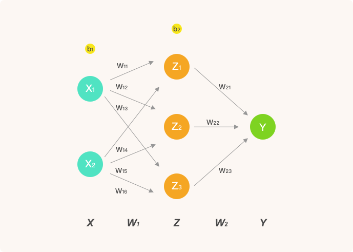
The neural network we plan to build contains 2 hidden layers, and the structure is as follows:
As you can see, the shape of the input data is \((N, 64)\), where \(N\) represents the number of samples. The neural network above has a total of 2 fully connected layers. The first layer processes the input data into \((N, 30)\), and then the second fully connected layer processes the training data into \((N, 10)\), which is directly used as the output layer for output. The output \((N, 10)\) exactly corresponds to the one-hot encoded target.
Specifically, we apply the ReLU activation function to the hidden layers and generally do not activate the output layer. At the same time, this time we include the bias term parameters and use randomly initialized tensor parameters.
import tensorflow as tf


class Model(object):
    def __init__(self):
        # 随机初始化张量参数
        self.W1 = tf.Variable(tf.random.normal([64, 30]))
        self.b1 = tf.Variable(tf.random.normal([30]))
        self.W2 = tf.Variable(tf.random.normal([30, 10]))
        self.b2 = tf.Variable(tf.random.normal([10]))

    def __call__(self, x):
        x = tf.cast(x, tf.float32)  # 转换输入数据类型
        # 线性计算 + RELU 激活
        fc1 = tf.nn.relu(tf.add(tf.matmul(x, self.W1), self.b1))  # 全连接层 1
        fc2 = tf.add(tf.matmul(fc1, self.W2), self.b2)  # 全连接层 2
        return fc2
The model class above must be familiar to everyone. It is
worth mentioning that
tf.cast
can not only convert the tensor type, but also directly
convert a NumPy array into a constant tensor of the
corresponding type. Remembering this will be very
convenient when using it.
52.5.3. Cross-entropy Loss Function#
After completing the construction of the forward propagation model, the next step is to define the loss function. Here, we choose a loss function that is very commonly used in the construction of deep neural networks: the cross-entropy loss function. The cross-entropy loss function is essentially the logarithmic loss function we learned before. Cross-entropy is mainly used to measure the difference information between two probability distributions. The cross-entropy loss function will continuously decrease as the probability of the correct class decreases, and the returned loss value will become larger and larger. The formula for the cross-entropy loss function is as follows:
Among them, \(y_i\) is the predicted probability distribution, and \(y'_i\) is the actual probability distribution, that is, the label matrix after one-hot encoding processing.
You might think that we can directly input the output of the last fully connected layer above into the cross-entropy loss function and then find the minimum value of the loss. The logic is correct, but here we will not directly input the output. Instead, we will process it through a function called the Softmax function.
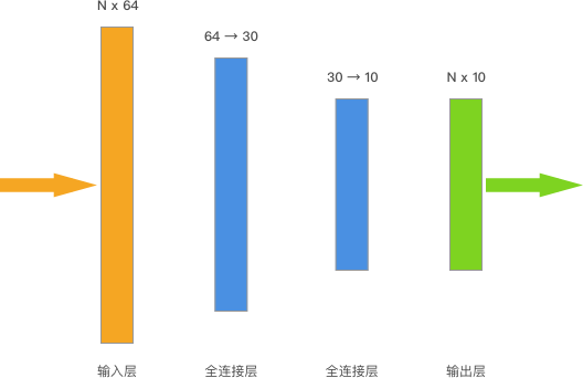
Therefore, let’s introduce the Softmax function, a very elegant and practical function. The formula for the Softmax function is as follows, and it can process numerical values into probabilities.
Simply put, we can convert the output of the fully connected layer into probabilities through this function, which is often used in classification problems. For example, if you see that the probability of predicting an animal to be a cat is 95.8%, it is very likely that the Softmax function is used.
For example, in the iris classification problem, if the last fully connected layer gives three outputs, which are -1.3, 2.6, and -0.9 respectively. After processing through the Softmax function, probability values of 0.02, 0.95, and 0.03 can be obtained. That is to say, there is a 95% probability that it belongs to the iris of the Versicolor category.
Of course, this also applies to the ten-class classification problem in our DIGITS this time, except that the above three classifications seem simpler. We can test whether it is the above output. Now, implement the Softmax function and test it:
def softmax(x):
    # Softmax 实现
    exp_x = np.exp(x)
    return exp_x / np.sum(exp_x)


np.round(softmax([-1.3, 2.6, -0.9]), 2)
array([0.02, 0.95, 0.03])
So the Softmax function is really very useful and can be seen in basically all classification models.
For ease of use, TensorFlow provides a combined API for
the cross-entropy loss function and the Softmax function:
tf.nn.softmax_cross_entropy_with_logits
🔗. Now we can directly use this function, where
logits
are the model outputs and
labels
are the true values of the samples. This API will return
the loss calculation results for each sample, so we will
use
tf.reduce_mean
🔗
to obtain the average value, thereby getting the loss on
the training set.
def loss_fn(model, x, y):
    preds = model(x)
    return tf.reduce_mean(
        tf.nn.softmax_cross_entropy_with_logits(logits=preds, labels=y)
    )
Let’s go back to a question left before: Why do we need to
perform one-hot encoding on the output values? This is
because we will use the Softmax function to process the
output of the fully connected layer into probabilities and
finally calculate the cross-entropy loss. And
tf.nn.softmax_cross_entropy_with_logits
naturally requires one-hot encoded data to be passed in.
With the loss function, the next step is to define an optimizer to find the minimum value of the global loss. Here we no longer use gradient descent, but the more commonly used Adam optimizer in deep learning. Adam is actually a mathematical optimization method, which was first proposed by Diederik P. Kingma et al. in 2014 🔗. The full name of Adam is Adaptive Moment Estimation. It is an algorithm with an adaptive learning rate, which calculates an adaptive learning rate for each parameter.
The experiment will no longer introduce the mathematical optimization process of Adam. You can directly call the Adam optimizer through TensorFlow. Now you can build and start performing iterative learning of the neural network.
EPOCHS = 200  # 迭代此时
LEARNING_RATE = 0.02  # 学习率
model = Model()  # 实例化模型类
for epoch in range(EPOCHS):
    with tf.GradientTape() as tape:  # 追踪梯度
        loss = loss_fn(model, X_train, y_train)

    trainable_variables = [model.W1, model.b1, model.W2, model.b2]  # 需优化参数列表
    grads = tape.gradient(loss, trainable_variables)  # 计算梯度

    optimizer = tf.optimizers.Adam(learning_rate=LEARNING_RATE)  # Adam 优化器
    optimizer.apply_gradients(zip(grads, trainable_variables))  # 更新梯度

    # 每 100 个 Epoch 输出各项指标
    if epoch == 0:
        print(f"Epoch [000/{EPOCHS}], Loss: [{loss:.4f}]")
    elif (epoch + 1) % 100 == 0:
        print(f"Epoch [{epoch+1}/{EPOCHS}], Loss: [{loss:.4f}]")
Epoch [000/200], Loss: [380.0146]
Epoch [100/200], Loss: [6.4553]
Epoch [200/200], Loss: [4.1002]
So far, we have completed the training of the DIGITS handwritten character recognition neural network according to the steps of building a neural network with standard TensorFlow.
At this point, you may have one last question, which is to
find out how well the network performs and need to print
out the classification accuracy of the network. Then, here
we need to define another accuracy calculation function.
First,
tf.math.argmax(y,
                        1)
🔗
returns the index with the maximum value on the tensor
axis from the true labels (one-hot encoded), thus
converting the Softmax result into the corresponding
character value. Then use
tf.equal
to compare whether the results of each sample are correct,
and finally use
reduce_mean
to obtain the classification accuracy of all samples.
def accuracy_fn(logits, labels):
    preds = tf.argmax(logits, axis=1)  # 取值最大的索引,正好对应字符标签
    labels = tf.argmax(labels, axis=1)
    return tf.reduce_mean(tf.cast(tf.equal(preds, labels), tf.float32))
Next, we re - execute the training process and print out the classification accuracy on the test set.
EPOCHS = 500  # 迭代此时
LEARNING_RATE = 0.02  # 学习率
model = Model()  # 实例化模型类
for epoch in range(EPOCHS):
    with tf.GradientTape() as tape:  # 追踪梯度
        loss = loss_fn(model, X_train, y_train)

    trainable_variables = [model.W1, model.b1, model.W2, model.b2]  # 需优化参数列表
    grads = tape.gradient(loss, trainable_variables)  # 计算梯度

    optimizer = tf.optimizers.Adam(learning_rate=LEARNING_RATE)  # Adam 优化器
    optimizer.apply_gradients(zip(grads, trainable_variables))  # 更新梯度

    accuracy = accuracy_fn(model(X_test), y_test)  # 计算准确度

    # 每 100 个 Epoch 输出各项指标
    if epoch == 0:
        print(f"Epoch [000/{EPOCHS}], Accuracy: [{accuracy:.2f}], Loss: [{loss:.4f}]")
    elif (epoch + 1) % 100 == 0:
        print(
            f"Epoch [{epoch+1}/{EPOCHS}], Accuracy: [{accuracy:.2f}], Loss: [{loss:.4f}]"
        )
Epoch [000/500], Accuracy: [0.09], Loss: [412.3293]
Epoch [100/500], Accuracy: [0.88], Loss: [3.4343]
Epoch [200/500], Accuracy: [0.89], Loss: [2.0059]
Epoch [300/500], Accuracy: [0.91], Loss: [1.2532]
Epoch [400/500], Accuracy: [0.91], Loss: [0.9231]
Epoch [500/500], Accuracy: [0.91], Loss: [0.7796]
It can be seen that after 500 iterations, the test set accuracy is approximately around 95%. (Due to the random initialization of parameters, the training results are slightly different each time)
52.6. Mini Batch Training Implementation with TensorFlow#
You may have noticed that when we trained the neural network above, we passed all the data into the network every time to optimize the parameters. Naturally, this is the best way, but when the amount of data is too large, the matrix calculations become quite exaggerated, and the memory occupied may even make training completely impossible. Therefore, in practice, a method called Mini Batch is often used, that is, the entire data is divided into small batches and put into the model for training.
There are many ways to implement mini - batches. Here we
present a very simple one. In this experiment, we use the
K - fold cross - validation
method provided by scikit - learn to divide the data into K
mini - batches. Briefly speaking, we can use
sklearn.model_selection.KFold
to divide the data into K equally - spaced chunks, and then
only select 1 chunk of data to pass in each time, which
exactly conforms to the idea of mini - batches.
from sklearn.model_selection import KFold
from tqdm.notebook import tqdm

EPOCHS = 500  # 迭代此时
BATCH_SIZE = 64  # 每次迭代的批量大小
LEARNING_RATE = 0.02  # 学习率

model = Model()  # 实例化模型类

for epoch in tqdm(range(EPOCHS)):  # 设定全数据集迭代次数
    indices = np.arange(len(X_train))  # 生成训练数据长度规则序列
    np.random.shuffle(indices)  # 对索引序列进行打乱,保证为随机数据划分
    batch_num = int(len(X_train) / BATCH_SIZE)  # 根据批量大小求得要划分的 batch 数量
    kf = KFold(n_splits=batch_num)  # 将数据分割成 batch 数量份
    # KFold 划分打乱后的索引序列,然后依据序列序列从数据中抽取 batch 样本
    for _, index in kf.split(indices):
        X_batch = X_train[indices[index]]  # 按打乱后的序列取出数据
        y_batch = y_train[indices[index]]

        with tf.GradientTape() as tape:  # 追踪梯度
            loss = loss_fn(model, X_batch, y_batch)

        trainable_variables = [model.W1, model.b1, model.W2, model.b2]  # 需优化参数列表
        grads = tape.gradient(loss, trainable_variables)  # 计算梯度

        optimizer = tf.optimizers.Adam(learning_rate=LEARNING_RATE)  # Adam 优化器
        optimizer.apply_gradients(zip(grads, trainable_variables))  # 更新梯度
        accuracy = accuracy_fn(model(X_test), y_test)  # 计算准确度

    # 每 100 个 Epoch 输出各项指标
    if epoch == 0:
        print(f"Epoch [000/{EPOCHS}], Accuracy: [{accuracy:.2f}], Loss: [{loss:.4f}]")
    elif (epoch + 1) % 100 == 0:
        print(
            f"Epoch [{epoch+1}/{EPOCHS}], Accuracy: [{accuracy:.2f}], Loss: [{loss:.4f}]"
        )
Epoch [000/500], Accuracy: [0.54], Loss: [23.4109]
Epoch [100/500], Accuracy: [0.94], Loss: [0.0000]
Epoch [200/500], Accuracy: [0.94], Loss: [0.0059]
Epoch [300/500], Accuracy: [0.95], Loss: [0.0000]
Epoch [400/500], Accuracy: [0.95], Loss: [0.0000]
Epoch [500/500], Accuracy: [0.95], Loss: [0.0000]
In the above code, since the
index
obtained from the KFold loop is always in sequential order,
we generated the sequential sequence
indices
of the data length in advance and then used
shuffle
to打乱 this sequence. Finally, we took the values from the
shuffled
indices
as the indices for fetching batches of training data.
The purpose of doing this is to ensure that the data of the mini - batches used in each Epoch iteration is different and to ensure that all the training data can be cycled through in one Epoch. It can be seen that the final accuracy of the mini - batch iteration is still good, and even better than that of the complete dataset iteration. Later, we will also learn to use the mini - batch method provided by TensorFlow to process data.
{note}
In the experiment, we use K - fold cross - validation provided by scikit - learn to implement mini - batch training in TensorFlow. You don't have to memorize this method. This is just for teaching demonstration. The key is to understand the process of mini - batch training. In most cases, we don't implement the mini - batch training process ourselves, but directly use the methods provided in the high - level API of TensorFlow.
In the above small example, there are two common terms: Batch and Epoch, which you will often see later. Batch, of course, is Mini Batch, that is, each time a small part is drawn from the dataset for training the neural network. Epoch refers to how many times the dataset is trained. An Epoch consists of a finite number of Batches.
Many people are easily confused about the difference between Batch and Epoch. You can learn to distinguish them through the following schematic diagram:

In addition, you can also read the article Epoch vs Batch Size vs Iterations [Requires scientific Internet access].
52.7. Summary#
In this experiment, we learned the classic methods and steps for building neural networks using TensorFlow, which must be firmly remembered. There are multiple commonly used functions and classes in the experiment, and you need to read the official documentation through the links to understand them in depth. You may feel that after learning so much, it seems not as simple as using the neural network class provided by scikit-learn. In fact, this is just the beginning of learning to build neural networks with TensorFlow. Subsequently, we will learn more user-friendly high-level APIs. In addition, scikit-learn cannot be used to build deep neural networks. You will understand later that it can only be completed using deep learning frameworks such as TensorFlow.
Related Links