
13. K-Nearest Neighbors Algorithm Implementation and Application#
13.1. Introduction#
In the process of solving classification problems, the K-Nearest Neighbors algorithm (abbreviated as: KNN) is a simple and practical method. This experiment will introduce the K-Nearest Neighbors algorithm in detail, and familiarize with the principle and Python implementation of the K-Nearest Neighbors algorithm from aspects such as distance calculation and classification decision-making. Finally, a prediction model will be constructed using the K-Nearest Neighbors algorithm to achieve the classification of lilacs.
13.2. Key Points#
Nearest Neighbor Algorithm
K-Nearest Neighbors Algorithm
Decision Rule
KNN Algorithm Implementation
13.3. Nearest Neighbor Algorithm#
Before introducing the K-Nearest Neighbors algorithm, let’s first talk about the Nearest Neighbor algorithm. The Nearest Neighbor algorithm (abbreviated as: NN) aims to find the training sample \(y\) in the training set that is most similar to the unknown class data \(x\) for the unknown class data \(x\), and use the class corresponding to the sample \(y\) as the class of the unknown class data \(x\), so as to achieve the classification effect.
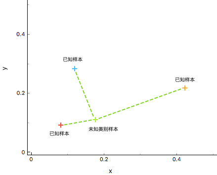
As shown in the figure above, by calculating the distances between the data \(X_{u}\) (unknown sample) and the known classes \({\omega_{1},\omega_{2},\omega_{3}}\) (known samples), the similarity between \(X_{u}\) and different training sets is judged, and finally the class of \(X_{u}\) is determined. Obviously, it is more appropriate to determine that the class of the green unknown sample is the same as that of the red known sample.
13.4. K-Nearest Neighbors Algorithm#
The K-Nearest Neighbors (abbreviated as: KNN) algorithm is a generalization of the Nearest Neighbor (NN) algorithm and is also one of the simplest methods in machine learning classification algorithms. The core idea of the KNN algorithm is similar to that of the Nearest Neighbor algorithm, both of which classify by finding the classes similar to the unknown samples. However, in the NN algorithm, only 1 sample is relied on for decision-making, which is too absolute in classification and will result in poor classification effects. To solve the defects of the NN algorithm, the KNN algorithm uses the method of K adjacent samples to jointly decide the class of the unknown sample. In this way, the error tolerance rate in decision-making is much higher than that of the NN algorithm, and the classification effect will also be better.
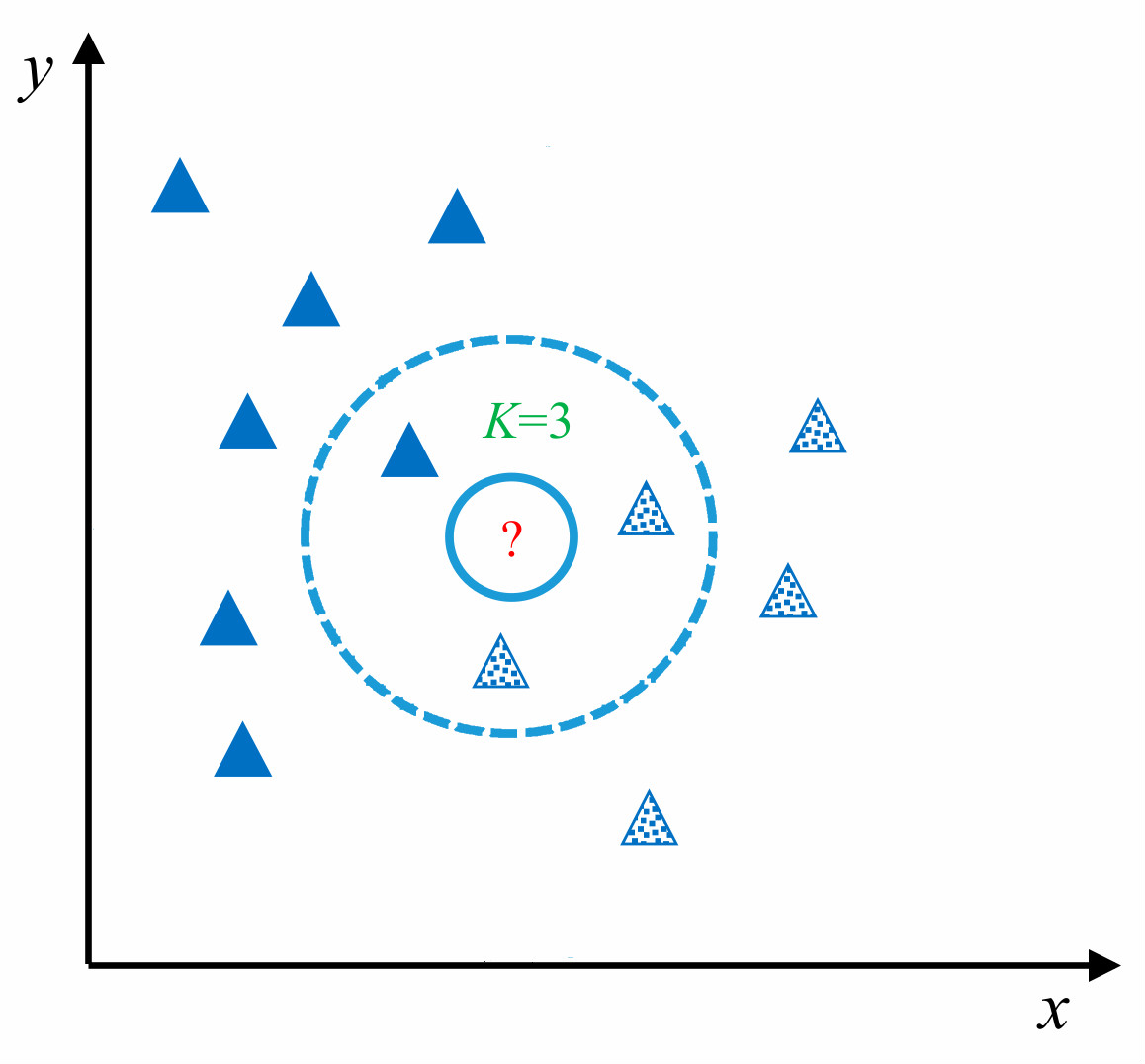
As shown in the figure above, for the unknown test sample (shown as ? in the figure), the KNN algorithm is used for classification. First, the similarity between the unknown sample and the training samples is calculated to find the nearest K adjacent samples (in the figure, the value of K is 3, and the 3 samples closest to?) are circled), and then the class of the unknown sample is finally determined based on the nearest K samples.
13.5. Implementation of K-Nearest Neighbors Algorithm#
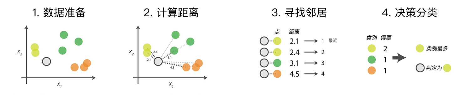
The KNN algorithm is very mature in theory. Its simple and easy-to-understand idea and good classification accuracy make the KNN algorithm widely used. The specific process of the algorithm mainly consists of the following 4 steps:
-
Data Preparation: Through data cleaning and data processing, each piece of data is organized into a vector.
-
Calculate Distance: Calculate the distance between the test data and the training data.
-
Find Neighbors: Find the K training data samples that are closest to the test data.
-
Decision Classification: According to the decision rule, obtain the class of the test data from the K neighbors.
Next, we try to complete a KNN classification process. First, generate a set of sample data, which contains two classes \(A\) and \(B\), and each piece of data contains two features \(x\) and \(y\).
import numpy as np


def create_data():
    features = np.array(
        [
            [2.88, 3.05],
            [3.1, 2.45],
            [3.05, 2.8],
            [2.9, 2.7],
            [2.75, 3.4],
            [3.23, 2.9],
            [3.2, 3.75],
            [3.5, 2.9],
            [3.65, 3.6],
            [3.35, 3.3],
        ]
    )
    labels = ["A", "A", "A", "A", "A", "B", "B", "B", "B", "B"]
    return features, labels
Then, we try to load and print this data.
features, labels = create_data()
print("features: \n", features)
print("labels: \n", labels)
features:
 [[2.88 3.05]
 [3.1  2.45]
 [3.05 2.8 ]
 [2.9  2.7 ]
 [2.75 3.4 ]
 [3.23 2.9 ]
 [3.2  3.75]
 [3.5  2.9 ]
 [3.65 3.6 ]
 [3.35 3.3 ]]
labels:
 ['A', 'A', 'A', 'A', 'A', 'B', 'B', 'B', 'B', 'B']
To understand the data more intuitively, next, use the
pyplot package in Matplotlib to visualize the dataset. For
the sake of code simplicity, we use the
map
function and
lambda
expressions to process the data. If you are not familiar
with these two methods, you need to teach yourself the
corresponding Python knowledge.
from matplotlib import pyplot as plt

%matplotlib inline

plt.figure(figsize=(5, 5))
plt.xlim((2.4, 3.8))
plt.ylim((2.4, 3.8))

x_feature = list(map(lambda x: x[0], features))  # 返回每个数据的x特征值
y_feature = list(map(lambda y: y[1], features))

plt.scatter(x_feature[:5], y_feature[:5], c="b")  # 在画布上绘画出"A"类标签的数据点
plt.scatter(x_feature[5:], y_feature[5:], c="g")
plt.scatter([3.18], [3.15], c="r", marker="x")  # 待测试点的坐标为 [3.1,3.2]
<matplotlib.collections.PathCollection at 0x117b3b430>

As shown in the figure above, the data with the label \(A\) (blue dots) is located in the lower left corner of the canvas, while the data with the label \(B\) (green dots) is in the upper right corner of the canvas. It can be clearly seen from the image the distribution of data with different labels. Among them, the red x points represent the test data whose category needs to be predicted in this experiment.
13.6. Distance Metric#
When calculating the similarity between two samples, it can be represented by calculating the distance of the feature values between the samples. If the distance value between two samples is larger (farther apart), it means that the similarity between the two samples is low. On the contrary, if the value of the two samples is smaller (closer), it means that the similarity between the two samples is higher.
There are many ways to calculate distance. This experiment introduces two of the most commonly used distance formulas: Manhattan distance and Euclidean distance. The calculation diagrams of these two distances are as follows:
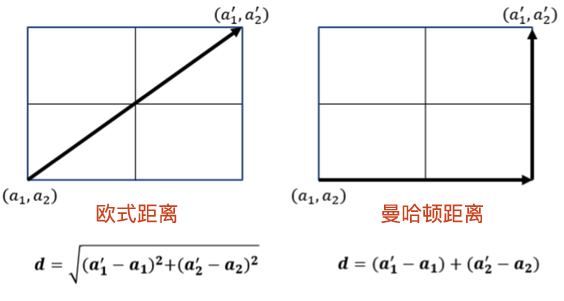
13.7. Manhattan Distance#
Manhattan distance, also known as Mahalanobis distance, is one of the simplest ways to calculate distance. The formula is as follows:
Where:
-
\(X\), \(Y\): Two data points
-
\(N\): There are \(N\) feature values in each data
-
\(X_{i}\): The \(i\)-th feature value of data \(X\)
The formula means that by taking the absolute value of the difference between each corresponding feature value in the two data points \(X\) and \(Y\) and then summing them up, the Manhattan distance is obtained.
def d_man(x, y):
    d = np.sum(np.abs(x - y))
    return d
x = np.array([3.1, 3.2])  # 任意指定 2 点计算
print("x:", x)

y = np.array([2.5, 2.8])
print("y:", y)

print(d_man(x, y))
x: [3.1 3.2]
y: [2.5 2.8]
1.0000000000000004
13.8. Euclidean Distance#
The Euclidean distance is derived from the distance formula between two points in an \(N\)-dimensional Euclidean space. The expression is as follows:
Where:
-
\(X\), \(Y\): Two data points
-
\(N\): There are \(N\) feature values in each data
-
\(X_{i}\): The \(i\)-th feature value of data \(X\)
The formula means that the Euclidean distance is obtained by taking the square of the difference between each corresponding feature value in the two data points \(X\) and \(Y\), summing them up, and finally taking the square root.
def d_euc(x, y):
    d = np.sqrt(np.sum(np.square(x - y)))
    return d
x = np.random.random(10)  # 随机生成 10 个数的数组作为 x 特征的值
print("x:", x)

y = np.random.random(10)
print("y:", y)

distance_euc = d_euc(x, y)
print(distance_euc)
x: [0.68561369 0.67904082 0.38730691 0.83837082 0.09327342 0.07623247
 0.20001211 0.3169432  0.15953875 0.48677777]
y: [0.99709904 0.65777056 0.13278858 0.2074084  0.43288451 0.35574441
 0.81063171 0.67753942 0.19673156 0.05628522]
1.2014259803870193
13.9. Decision Rules#
After obtaining the similarity between the test samples and the training samples, through the ranking of the similarities, the K nearest training samples for each test sample can be obtained. Then, how to determine the final category of the test sample based on these K neighbors? The decision rules can be selected according to the data characteristics. Different decision rules will produce different prediction results. The most commonly used decision rules are:
-
Majority Voting Method: The majority voting method is similar to the voting process, that is, to select the category with the largest number of occurrences among the K neighbors as the category of the test sample.
-
Weighted Voting Method: According to the distance, the votes of the neighbors are weighted. The closer the distance, the greater the weight. The category with the maximum value of the weighted calculation result is the category of the test sample.
We recommend using the majority voting method here. This method is simpler. The previous illustration in this experiment is the majority voting method.
import operator


def majority_voting(class_count):
    # 多数表决函数
    sorted_class_count = sorted(
        class_count.items(), key=operator.itemgetter(1), reverse=True
    )
    return sorted_class_count


arr = {"A": 3, "B": 2, "C": 6, "D": 5}
majority_voting(arr)
[('C', 6), ('D', 5), ('A', 3), ('B', 2)]
In the definition of the majority voting method, we imported
the
operator
calculation module, aiming to sort the dictionary type
structure. It can be seen from the result that the result
returned by the function is
C
with the most votes, and the number of votes is
6
times.
13.10. KNN Algorithm Implementation#
After learning the above steps, the KNN algorithm is
gradually outlined. The following is the complete
implementation of the KNN algorithm. In this experiment, the
Euclidean distance is used for distance calculation, and the
decision rule for classification is the majority voting
method. Define the function
knn_classify(), and the parameters of the function include:
-
test_data: The input vector for classification. -
train_data: The input training sample set. -
labels: The class label vector of the sample data. -
k: The number of nearest neighbors to select.
def knn_classify(test_data, train_data, labels, k):
    # KNN 方法完整实现
    distances = np.array([])  # 创建一个空的数组用于存放距离

    for each_data in train_data:  # 使用欧式距离计算数据相似度
        d = d_euc(test_data, each_data)
        distances = np.append(distances, d)

    sorted_distance_index = distances.argsort()  # 获取按距离从小到大排序后的索引
    sorted_distance = np.sort(distances)
    r = (sorted_distance[k] + sorted_distance[k - 1]) / 2  # 计算

    class_count = {}
    for i in range(k):  # 多数表决
        vote_label = labels[sorted_distance_index[i]]
        class_count[vote_label] = class_count.get(vote_label, 0) + 1

    final_label = majority_voting(class_count)
    return final_label, r
13.11. Classification Prediction#
After implementing the KNN algorithm, we can then start
classifying our unknown data
[3.18,
                      3.15]
. Assuming our initial value of K is set to 5, let’s see
the classification results.
test_data = np.array([3.18, 3.15])
final_label, r = knn_classify(test_data, features, labels, 5)
final_label
[('B', 3), ('A', 2)]
13.12. Visualization#
After classifying the data
[3.18,
                      3.15]
, next we will also use a graphical method to visually
demonstrate the decision-making method of the KNN algorithm.
def circle(r, a, b):  # 为了画出圆,这里采用极坐标的方式对圆进行表示 :x=r*cosθ,y=r*sinθ。
    theta = np.arange(0, 2 * np.pi, 0.01)
    x = a + r * np.cos(theta)
    y = b + r * np.sin(theta)
    return x, y
k_circle_x, k_circle_y = circle(r, 3.18, 3.15)

plt.figure(figsize=(5, 5))
plt.xlim((2.4, 3.8))
plt.ylim((2.4, 3.8))

x_feature = list(map(lambda x: x[0], features))  # 返回每个数据的 x 特征值
y_feature = list(map(lambda y: y[1], features))

plt.scatter(x_feature[:5], y_feature[:5], c="b")  # 在画布上绘画出"A"类标签的数据点
plt.scatter(x_feature[5:], y_feature[5:], c="g")
plt.scatter([3.18], [3.15], c="r", marker="x")  # 待测试点的坐标为 [3.1,3.2]
plt.plot(k_circle_x, k_circle_y)
[<matplotlib.lines.Line2D at 0x117bce200>]

As shown in the figure, when our value of K is 5, among the 5 training data points closest to the test sample (shown as blue circles), 3 belong to class \(B\) and 2 belong to class \(A\). According to the majority voting method, the test sample is determined to be of class \(B\).
In the KNN algorithm, the choice of the value of K has a
great impact on the final decision of the data. Next, we
introduce the
ipywidgets
module to more clearly reflect the influence of the choice
of K on the prediction results. The
ipywidgets
module is an interactive module in
jupyter. Different values of K can be selected through a dropdown
menu to make judgments and predict the final category of
unknown points.
from ipywidgets import interact, fixed


def change_k(test_data, features, k):
    final_label, r = knn_classify(test_data, features, labels, k)
    k_circle_x, k_circle_y = circle(r, 3.18, 3.15)

    plt.figure(figsize=(5, 5))
    plt.xlim((2.4, 3.8))
    plt.ylim((2.4, 3.8))

    x_feature = list(map(lambda x: x[0], features))  # 返回每个数据的 x 特征值
    y_feature = list(map(lambda y: y[1], features))

    plt.scatter(x_feature[:5], y_feature[:5], c="b")  # 在画布上绘画出"A"类标签的数据点
    plt.scatter(x_feature[5:], y_feature[5:], c="g")
    plt.scatter([3.18], [3.15], c="r", marker="x")  # 待测试点的坐标为 [3.1,3.2]
    plt.plot(k_circle_x, k_circle_y)
interact(
    change_k, test_data=fixed(test_data), features=fixed(features), k=[3, 5, 7, 9]
)  # 可交互式绘图
<function __main__.change_k(test_data, features, k)>
It can be intuitively seen from the figure that different values of K predict different results. Next, we use the KNN algorithm to classify and predict a real dataset.
13.13. Load the dataset#
The dataset used this time is the Syringa dataset
course-9-syringa.csv. The Syringa dataset contains 3 categories such as
daphne,
syringa, and
willow. Each category contains 150 data entries, and each data
entry contains 4 feature values: sepal length, sepal width,
petal length, and petal width. Use Pandas to import it into
a DataFrame format.
wget -nc https://cdn.aibydoing.com/aibydoing/files/course-9-syringa.csv
import pandas as pd

lilac_data = pd.read_csv("course-9-syringa.csv")
lilac_data.head()  # 预览前 5 行
| sepal_length | sepal_width | petal_length | petal_width | labels | |
|---|---|---|---|---|---|
| 0 | 5.1 | 3.5 | 2.4 | 2.1 | daphne |
| 1 | 4.9 | 3.0 | 2.7 | 1.7 | daphne |
| 2 | 4.7 | 3.2 | 2.2 | 1.4 | daphne |
| 3 | 4.6 | 3.1 | 1.6 | 1.7 | daphne |
| 4 | 5.0 | 3.6 | 1.6 | 1.4 | daphne |
To better understand the data, we also use
plt
to plot the features of each data entry. Since the Syringa
dataset has 4 feature values and cannot be directly
represented in a two-dimensional space, we have to draw the
feature distribution map by combining features. Next, we
combine the 4 features in pairs to get 6 cases and use
subplots to draw them.
"""绘制丁香花特征子图
"""
fig, axes = plt.subplots(2, 3, figsize=(20, 10))  # 构建生成 2*3 的画布,2 行 3 列
fig.subplots_adjust(hspace=0.3, wspace=0.2)  # 定义每个画布内的行间隔和高间隔

axes[0, 0].set_xlabel("sepal_length")  # 定义 x 轴坐标值
axes[0, 0].set_ylabel("sepal_width")  # 定义 y 轴坐标值
axes[0, 0].scatter(lilac_data.sepal_length[:50], lilac_data.sepal_width[:50], c="b")
axes[0, 0].scatter(
    lilac_data.sepal_length[50:100], lilac_data.sepal_width[50:100], c="g"
)
axes[0, 0].scatter(lilac_data.sepal_length[100:], lilac_data.sepal_width[100:], c="r")
axes[0, 0].legend(["daphne", "syringa", "willow"], loc=2)  # 定义示例

axes[0, 1].set_xlabel("petal_length")
axes[0, 1].set_ylabel("petal_width")
axes[0, 1].scatter(lilac_data.petal_length[:50], lilac_data.petal_width[:50], c="b")
axes[0, 1].scatter(
    lilac_data.petal_length[50:100], lilac_data.petal_width[50:100], c="g"
)
axes[0, 1].scatter(lilac_data.petal_length[100:], lilac_data.petal_width[100:], c="r")

axes[0, 2].set_xlabel("sepal_length")
axes[0, 2].set_ylabel("petal_length")
axes[0, 2].scatter(lilac_data.sepal_length[:50], lilac_data.petal_length[:50], c="b")
axes[0, 2].scatter(
    lilac_data.sepal_length[50:100], lilac_data.petal_length[50:100], c="g"
)
axes[0, 2].scatter(lilac_data.sepal_length[100:], lilac_data.petal_length[100:], c="r")

axes[1, 0].set_xlabel("sepal_width")
axes[1, 0].set_ylabel("petal_width")
axes[1, 0].scatter(lilac_data.sepal_width[:50], lilac_data.petal_width[:50], c="b")
axes[1, 0].scatter(
    lilac_data.sepal_width[50:100], lilac_data.petal_width[50:100], c="g"
)
axes[1, 0].scatter(lilac_data.sepal_width[100:], lilac_data.petal_width[100:], c="r")

axes[1, 1].set_xlabel("sepal_length")
axes[1, 1].set_ylabel("petal_width")
axes[1, 1].scatter(lilac_data.sepal_length[:50], lilac_data.petal_width[:50], c="b")
axes[1, 1].scatter(
    lilac_data.sepal_length[50:100], lilac_data.petal_width[50:100], c="g"
)
axes[1, 1].scatter(lilac_data.sepal_length[100:], lilac_data.petal_width[100:], c="r")

axes[1, 2].set_xlabel("sepal_width")
axes[1, 2].set_ylabel("petal_length")
axes[1, 2].scatter(lilac_data.sepal_width[:50], lilac_data.petal_length[:50], c="b")
axes[1, 2].scatter(
    lilac_data.sepal_width[50:100], lilac_data.petal_length[50:100], c="g"
)
axes[1, 2].scatter(lilac_data.sepal_width[100:], lilac_data.petal_length[100:], c="r")
<matplotlib.collections.PathCollection at 0x1311d66b0>

Since this dataset has many features, the data distribution is presented by combining features. When encountering more features, data analysis can also be carried out by reducing the dimensionality of data features, and the corresponding methods will be explained in subsequent courses.
13.14. Training and Testing Data Division#
When obtaining a dataset and hoping to get a training model from it, we often split the data into two parts, one part is the training set and the other part is the test set. According to experience, a better splitting method is random splitting, and the splitting ratio is: 70% as the training set and 30% as the test set.
Here we use the
train_test_split
function of the scikit-learn module to complete the
splitting of the dataset.
from sklearn.model_selection import train_test_split

X_train,X_test, y_train, y_test =train_test_split(train_data,train_target,test_size=0.4, random_state=0)
Among them:
-
X_train,X_test,y_train, andy_testrespectively represent the training set of features after splitting, the test set of features, the training set of labels, and the test set of labels; where the values of features and labels correspond one by one. -
train_dataandtrain_targetrespectively represent the feature set to be divided and the label set to be divided. -
test_size: The proportion of test samples. -
random_state: Random number seed. When repeated experiments are required, it ensures that the same set of random numbers can be obtained when the random number seeds are the same.
from sklearn.model_selection import train_test_split

# 得到 lilac 数据集中 feature 的全部序列: sepal_length,sepal_width,petal_length,petal_width
feature_data = lilac_data.iloc[:, :-1]
label_data = lilac_data["labels"]  # 得到 lilac 数据集中 label 的序列

X_train, X_test, y_train, y_test = train_test_split(
    feature_data, label_data, test_size=0.3, random_state=2
)

X_test  # 输出 lilac_test 查看
| sepal_length | sepal_width | petal_length | petal_width | |
|---|---|---|---|---|
| 6 | 4.6 | 3.4 | 2.5 | 1.6 |
| 3 | 4.6 | 3.1 | 1.6 | 1.7 |
| 113 | 5.1 | 2.5 | 4.6 | 2.0 |
| 12 | 4.8 | 3.0 | 2.2 | 1.5 |
| 24 | 4.8 | 3.4 | 2.1 | 2.2 |
| 129 | 6.2 | 3.0 | 4.0 | 1.6 |
| 25 | 5.0 | 3.0 | 3.3 | 1.7 |
| 108 | 5.7 | 2.5 | 4.1 | 2.8 |
| 128 | 5.9 | 2.8 | 4.1 | 2.1 |
| 45 | 4.8 | 3.0 | 1.9 | 1.5 |
| 48 | 5.3 | 3.7 | 3.0 | 1.8 |
| 42 | 4.4 | 3.2 | 2.1 | 1.3 |
| 35 | 5.0 | 3.2 | 1.4 | 1.3 |
| 5 | 5.4 | 3.9 | 1.8 | 1.5 |
| 85 | 6.0 | 3.4 | 4.5 | 1.7 |
| 54 | 6.5 | 2.8 | 4.6 | 2.4 |
| 41 | 4.5 | 2.3 | 2.5 | 1.3 |
| 96 | 5.7 | 2.9 | 4.2 | 2.3 |
| 144 | 6.7 | 3.3 | 4.9 | 2.5 |
| 89 | 5.5 | 2.5 | 4.0 | 2.2 |
| 77 | 6.7 | 3.0 | 5.0 | 2.1 |
| 74 | 6.4 | 2.9 | 4.3 | 1.9 |
| 115 | 6.3 | 3.2 | 4.2 | 2.3 |
| 94 | 5.6 | 2.7 | 4.2 | 1.5 |
| 87 | 6.3 | 2.3 | 4.4 | 1.8 |
| 29 | 4.7 | 3.2 | 2.4 | 1.7 |
| 2 | 4.7 | 3.2 | 2.2 | 1.4 |
| 127 | 6.1 | 3.0 | 3.5 | 1.8 |
| 44 | 5.1 | 3.8 | 3.1 | 2.7 |
| 125 | 6.5 | 3.2 | 5.7 | 1.8 |
| 126 | 5.3 | 2.8 | 4.3 | 1.8 |
| 23 | 5.1 | 3.3 | 2.1 | 2.0 |
| 64 | 5.6 | 2.9 | 3.6 | 1.7 |
| 117 | 7.5 | 3.8 | 4.9 | 2.2 |
| 84 | 5.4 | 3.0 | 4.5 | 2.2 |
| 14 | 5.8 | 4.0 | 2.4 | 1.5 |
| 132 | 5.4 | 2.8 | 4.0 | 2.2 |
| 91 | 6.1 | 3.0 | 4.6 | 1.4 |
| 53 | 5.5 | 2.3 | 4.0 | 1.8 |
| 141 | 6.7 | 3.1 | 3.6 | 2.3 |
| 78 | 6.0 | 2.9 | 4.5 | 1.7 |
| 97 | 6.2 | 2.9 | 4.3 | 2.3 |
| 143 | 5.9 | 3.2 | 4.5 | 2.3 |
| 93 | 5.0 | 2.3 | 3.3 | 1.8 |
| 11 | 4.8 | 3.4 | 2.2 | 1.7 |
13.15. Train the Model#
In the previous experimental section, we have implemented the KNN algorithm according to the process using Python. In actual combat, we more often use the KNN function in the scikit-learn library to implement data classification.
sklearn.neighbors.KNeighborsClassifier((n_neighbors=5, weights='uniform', algorithm='auto')
Among them:
-
n_neighbors: The value ofk, representing the number of neighbors, with a default value of5. -
weights: The decision rule selection, either majority voting or weighted voting, with available parameters ('uniform','distance'). -
algorithm: The search algorithm selection (auto,kd_tree,ball_tree), including brute-force search,kd-tree search, orball-tree search.
from sklearn.neighbors import KNeighborsClassifier


def sklearn_classify(train_data, label_data, test_data, k_num):
    # 使用 sklearn 构建 KNN 预测模型
    knn = KNeighborsClassifier(n_neighbors=k_num)
    # 训练数据集
    knn.fit(train_data, label_data)
    # 预测
    predict_label = knn.predict(test_data)
    # 返回预测值
    return predict_label
13.16. Model Prediction#
After defining the function above, the next step is to
classify the test set separated from the lilac dataset. Pass
in
X_train,
y_train,
X_test, and the K value of 3. After classification using the KNN
algorithm, output the classification results of the test
set.
# 使用测试数据进行预测
y_predict = sklearn_classify(X_train, y_train, X_test, 3)
y_predict
array(['daphne', 'daphne', 'willow ', 'daphne', 'daphne', 'willow ',
       'daphne', 'syringa', 'willow ', 'daphne', 'daphne', 'daphne',
       'daphne', 'daphne', 'syringa', 'syringa', 'syringa', 'willow ',
       'syringa', 'willow ', 'syringa', 'willow ', 'willow ', 'syringa',
       'syringa', 'daphne', 'daphne', 'willow ', 'daphne', 'willow ',
       'willow ', 'daphne', 'syringa', 'willow ', 'willow ', 'daphne',
       'willow ', 'willow ', 'syringa', 'willow ', 'willow ', 'willow ',
       'willow ', 'syringa', 'daphne'], dtype=object)
13.17. Accuracy Calculation#
After obtaining the prediction results, we need to evaluate the performance of the model, that is, to obtain the accuracy of the model prediction. Calculating the accuracy is to compare the differences between the predicted values and the true values, obtain the number of samples with correct predictions, and divide it by the total number of the test set.
def get_accuracy(test_labels, pred_labels):
    # 准确率计算函数
    correct = np.sum(test_labels == pred_labels)  # 计算预测正确的数据个数
    n = len(test_labels)  # 总测试集数据个数
    accur = correct / n
    return accur
Through the above accuracy calculation function, the classification accuracy of the test data can be obtained according to the following code.
get_accuracy(y_test, y_predict)
0.7777777777777778
13.18. K Value Selection#
When the value of K is selected as 3, it can be seen that the accuracy is not high and the classification effect is not very satisfactory. The selection of the value of K has always been a hot topic and there has not been a good solution so far. According to experience, the value of K is preferably not more than the square root of the number of samples. Therefore, a suitable value of K can be selected by traversing. Here, we plot the accuracy for each value of K from 2 to 10 to obtain the optimal value of K.
normal_accuracy = []  # 建立一个空的准确率列表
k_value = range(2, 11)
for k in k_value:
    y_predict = sklearn_classify(X_train, y_train, X_test, k)
    accuracy = get_accuracy(y_test, y_predict)
    normal_accuracy.append(accuracy)

plt.xlabel("k")
plt.ylabel("accuracy")
new_ticks = np.linspace(0.6, 0.9, 10)  # 设定 y 轴显示,从 0.6 到 0.9
plt.yticks(new_ticks)
plt.plot(k_value, normal_accuracy, c="r")
plt.grid(True)  # 给画布增加网格

From the image, it can be obtained that when K = 4 and K = 6, the model accuracies are quite similar. However, when selecting the optimal model in machine learning, we generally consider the generalization ability of the model. Therefore, here we choose K = 4, which is the simpler model.
13.19. Kd - Tree#
The ease of understanding of the KNN algorithm is largely due to the fact that when classifying input examples in the implementation of KNN, the method used is linear scanning, that is, the input example calculates the distance with each training example. For this reason, when the amount of data is extremely large, such calculations will be very time-consuming. To improve the search efficiency of KNN and reduce the number of distance calculations, the computational efficiency can be improved by constructing a Kd-tree.
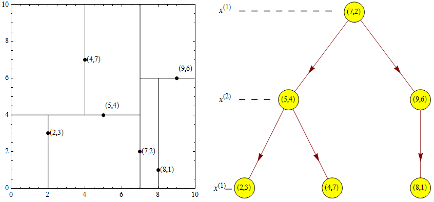
A Kd-tree (English: K-dimension tree) is a tree-shaped data structure for storing instance points in a K-dimensional space for quick retrieval. A Kd-tree is a binary tree that represents a partition of a K-dimensional space. Constructing a Kd-tree is equivalent to continuously dividing the K-dimensional space with hyperplanes perpendicular to the coordinate axes, forming a series of K-dimensional hyper-rectangular regions. Each node of the Kd-tree corresponds to a K-dimensional hyper-rectangular region. Using a Kd-tree can eliminate the search for most data points, thereby reducing the computational effort of the search.
13.20. Kd-tree Nearest Neighbor Search#
The following are the steps for the nearest neighbor search of a Kd-tree:
-
Start from the root node and move down recursively. The method of deciding whether to go left or right is the same as the method of inserting elements (if the input point is on the left side of the partition plane, enter the left child node; if it is on the right side, enter the right child node).
-
Once reaching a leaf node, regard this node as the “current best point”.
-
Unwind the recursion and perform the following steps for each node passed through:
-
If the current point is closer to the input point than the current best point, change it to the current best point.
-
Check if there is a closer point in the other subtree. If so, search down from that node.
-
-
When the search of the root node is completed, the nearest neighbor search is finished.
It can be intuitively found through the steps that compared with the traditional KNN search traversal, it saves a lot of time and space.
13.21. Kd-tree Implementation#
In the previous explanation, the main purpose of the Kd-tree
is to improve the speed of data search and reduce the
consumption of memory and time. Next, let’s intuitively
experience the advantages of the Kd-tree through code.
Implementing the Kd-tree using the scikit-learn library is
very simple. You only need to pass in the
kd_tree
parameter when calling the function.
In fact, the method provided by scikit-learn is no longer an
ordinary KNN implementation, but integrates a variety of
optimized search methods. Therefore, it is impossible to
compare the time with and without using the Kd-tree search
here. The default
algorithm='auto'
parameter will automatically select the optimized search
method to reduce the training time.
kd_x = np.random.random((100000, 2))  # 生成 10 万条测试数据
kd_y = np.random.randint(4, size=(100000))

kd_knn = KNeighborsClassifier(n_neighbors=5, algorithm="kd_tree")  # kd 树搜索
%time kd_knn.fit(kd_x, kd_y) # 输出 kd 树搜索训练用时
CPU times: user 88.7 ms, sys: 2.64 ms, total: 91.4 ms
Wall time: 32.3 ms
KNeighborsClassifier(algorithm='kd_tree')In a Jupyter environment, please rerun this cell to show the HTML representation or trust the notebook.
On GitHub, the HTML representation is unable to render, please try loading this page with nbviewer.org.
KNeighborsClassifier(algorithm='kd_tree')
13.22. Summary#
In this section of the experiment, we learned the principle and Python implementation of the KNN algorithm, as well as the implementation of the KNN algorithm using the scikit-learn library. Although the principle and logic of the KNN algorithm are simple, it performs very well in many classification or regression examples.
Related Links