
86. Implementation of Q-Learning Reinforcement Learning Method#
86.1. Introduction#
In the field of reinforcement learning methods, value-based reinforcement learning methods are a very important branch. In this experiment, starting from a case, two representative value-based reinforcement learning methods, Q-Learning and Sarsa, will be introduced in detail, and the Python implementation of Q-Learning will be carried out in combination with the algorithm process.
86.2. Key Points#
Concept of Q-Table
Implementation of Q-Learning Algorithm
Sarsa Learning Algorithm
Differences between Sarsa and Q-Learning
86.3. Classification of Reinforcement Learning Algorithms#
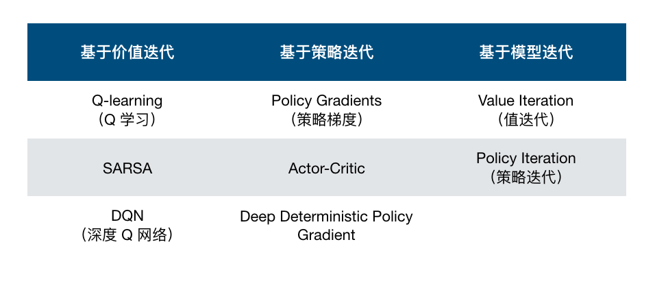
Previously, we presented the following classification table of reinforcement learning algorithms. This table classifies common reinforcement learning algorithms from three dimensions: value iteration-based, policy iteration-based, and model iteration-based. So, how are these three dimensions determined?
To answer the above question, we have to go back to the illustration of the reinforcement learning process to explain.
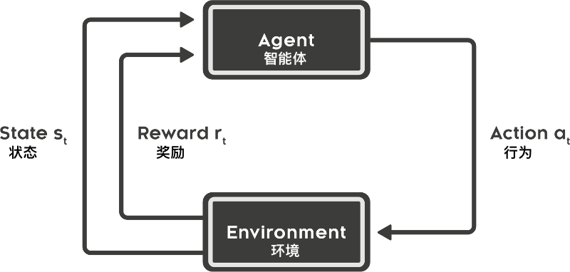
The above figure presents a typical reinforcement learning process, and we have elaborated on the five elements in the first introductory lesson. This time, we will explore the composition of the agent again.
In fact, the agent usually contains the following three components, which are:
-
Policy function: The behavior of the agent, which reflects the actions the agent can take. Among them, the state is used as the input, and its next action decision is used as the output.
-
Value function: It judges the quality of each state or action, similar to evaluating the expected reward after taking a certain action.
-
Model: The model is used for the agent to perceive the changes in the environment.
For the above three components, the agent does not need to have all of them every time. It can have one or more of them. And it is based on these three components that we get the three classification dimensions in the reinforcement learning algorithm classification table.
Therefore, a more rigorous classification of reinforcement learning algorithms is as follows:
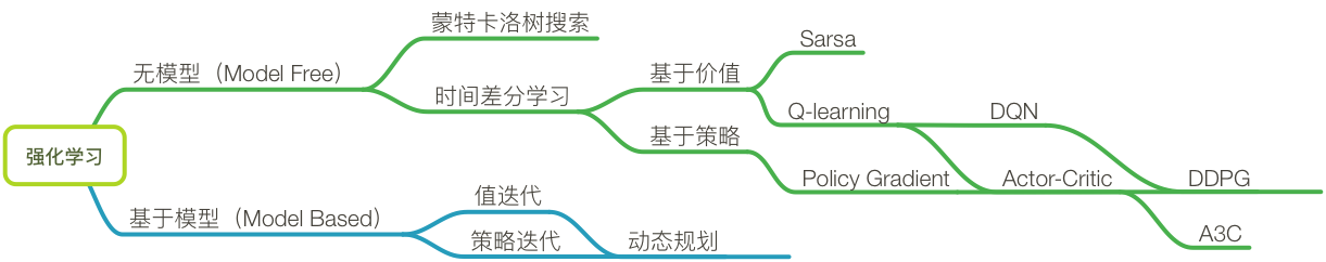
As shown in the figure above, based on Markov decision processes (MDPs), model-based and model-free reinforcement learning methods have evolved. And all the courses of this reinforcement learning focus on the part of temporal difference learning, and emphasize three of the most basic methods: Q-learning, Sarsa, and Policy Gradient.
86.4. Overview of Value-Based Reinforcement Learning#
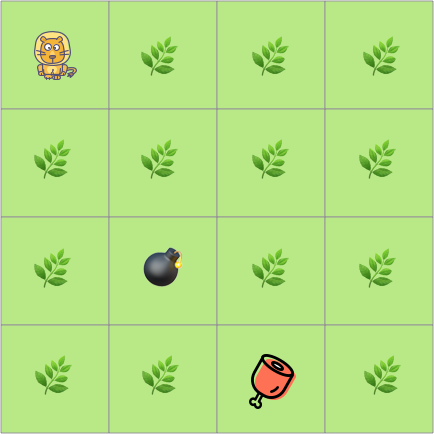
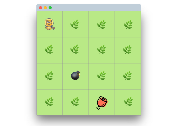
Suppose there is such a game scenario: A little lion is playing happily on the grassland. It knows that every time a kind-hearted person will place its favorite big ham at a fixed location. It hopes to quickly find the big ham, but there are many traps between its location and the place where the ham is placed. Once it touches a trap, the game ends, and the little lion has to start looking for a suitable path from the beginning. So how can the little lion find the big ham as soon as possible?
The stupidest method: The little lion knows and remembers the locations of the traps through attempts, and then, while avoiding the traps, looks for the safe lawn until it finds the big ham. Obviously, it is not advisable to try to find the shortest path randomly. So, apart from this, is there any other good way to solve this problem?
First, let’s think about what we would do in real life when we encounter an unfamiliar environment?
The most conventional method is of course to make marks: Record the possible benefits Q (safety or rewards) of exploring in four directions (up, down, left, right) on the lawns passed by. At first, we may move randomly and make marks. When we encounter a trap, we will change the marks to give ourselves a reminder. As the marks increase, we will choose the next action according to the marks (Q values), and then update the Q values on the lawn according to the results after the action.
Just like this, through repeated self-learning, marks will eventually be made on the entire lawn. In fact, the process of updating the marks (Q values) is the process of getting familiar with the environment. In subsequent attempts, the destination can be quickly found through these marks.
What would happen if we applied the thinking mode in real life to the game scenario we assumed? In fact, the Q value for making marks is the value (Quality), and the repeated self-learning based on the Q value is value-based reinforcement learning.
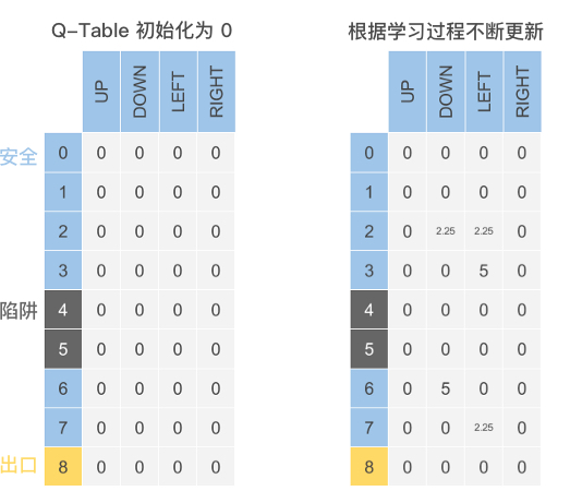
86.5. The Concept of Q-Table#
In the above case, when combining the game scenario with the five elements of reinforcement learning, it is easy to make one-to-one correspondences: The little lion is the Agent, the lawn is the Environment, each move is the Action, the state when moving to each lawn is the State, and the feedback when moving to the corresponding place is the Reward.
Combining the Q values of the marks made on all the lawns forms a table, which is called the Q-value table (Q-Table). In fact, the Q-Table is the core of the value-based reinforcement learning algorithm. Because in value-based reinforcement learning, the Q-Table can be used to determine the selection of actions, and the environmental feedback (Reward) obtained after the execution of the actions aims to update the Q-Table.
So, what exactly does the Q-Table look like?
As shown in the figure below (the data is randomly exemplified), the columns in the Q-Table are the selectable Action actions, and each row of data consists of the State states corresponding to the execution of different Actions. The data stored is the maximum expected reward value (Q value).
86.6. Q-Learning Learning Algorithm#
In value-based reinforcement learning, the most basic algorithms are Q-Learning and Sarsa, among which Q-Learning is a more widely used algorithm in practice. Similar to the method of the little lion looking for the big ham in the case, the principle of the Q-Learning algorithm is briefly described as follows:
-
Initialize the Q-Table: Construct a table with the same dimension according to the environment and the types of actions.
-
Action selection: Select actions based on the values in the Q-Table.
-
Action feedback: Obtain the action feedback given by the environment after taking an action.
-
Q-Table update: Update the Q-Table according to the feedback and the estimated future rewards.
Then, repeat steps 2 to 4 until the expected result is achieved or the pre-set number of iterations ends. Output the Q-Table to complete the Q-Learning learning process.
According to the algorithm principle of Q-Learning, below we use Python to restore the game scenario of the little lion looking for the big ham, and use the Q-Learning algorithm to help the little lion find the big ham as soon as possible.
86.7. Q-Learning Algorithm Implementation#
As previously mentioned, the entire process of reinforcement learning is completed in an environment. Therefore, we need to build an environment that can be used for algorithm testing, which is also what makes reinforcement learning different.
We want to test using the Q-Learning algorithm in a maze to help the little lion find the big ham as soon as possible. In a local environment, we can use Tkinter, PyQt, and wxPython supported by Python to write a GUI program, and the前期 process is rather complex. (这里“前期过程”直接用拼音qianqi process 不太合适,可考虑改为“前期流程”:preliminary process )修改后:We want to test using the Q-Learning algorithm in a maze to help the little lion find the big ham as soon as possible. In a local environment, we can use Tkinter, PyQt, and wxPython supported by Python to write a GUI program, and the preliminary process is rather complex.
In this experiment, for a more intuitive understanding and
also to support Jupyter Notebook, we simplify the maze game
of the little lion looking for the ham into a text version.
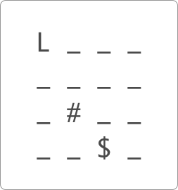
In the text game shown below, the little lion is represented
by
L, the trap is represented by
#, the big ham is represented by
$, and the ordinary lawn is represented by
_.
Next, we first use Python to complete the writing of the environment. You don’t need to master this part of the code. Just focus on understanding the code related to the reinforcement learning algorithm in this experiment.
import pandas as pd
import numpy as np
import time
from IPython import display  # 引入 display 模块目的方便程序运行展示


def init_env():
    start = (0, 0)
    terminal = (3, 2)
    hole = (2, 1)
    env = np.array([["_ "] * 4] * 4)  # 建立一个 4*4 的环境
    env[terminal] = "$ "  # 目的地
    env[hole] = "# "  # 陷阱
    env[start] = "L "  # 小狮子
    interaction = ""
    for i in env:
        interaction += "".join(i) + "\n"
    print(interaction)


init_env()
L _ _ _
_ _ _ _
_ # _ _
_ _ $ _
As can be seen, as shown in the schematic diagram, the environment of the text maze game has been created.
86.8. Initialize the Q-Table#
According to the actual environment, draw a
\(4*4\)
Q-Table. Divide the space for four directions of
up,
down,
left, and
right
in each cell. In fact, it is a
\(4*4*4\)
table, that is, 4 rows, 4 columns, and the height is 4 (four
different action directions). To observe the Q-Table more
intuitively, we define the Q-Table in the form of a
two-dimensional table
\(16*4\).
The column name is Action, and each State is represented by
a row.
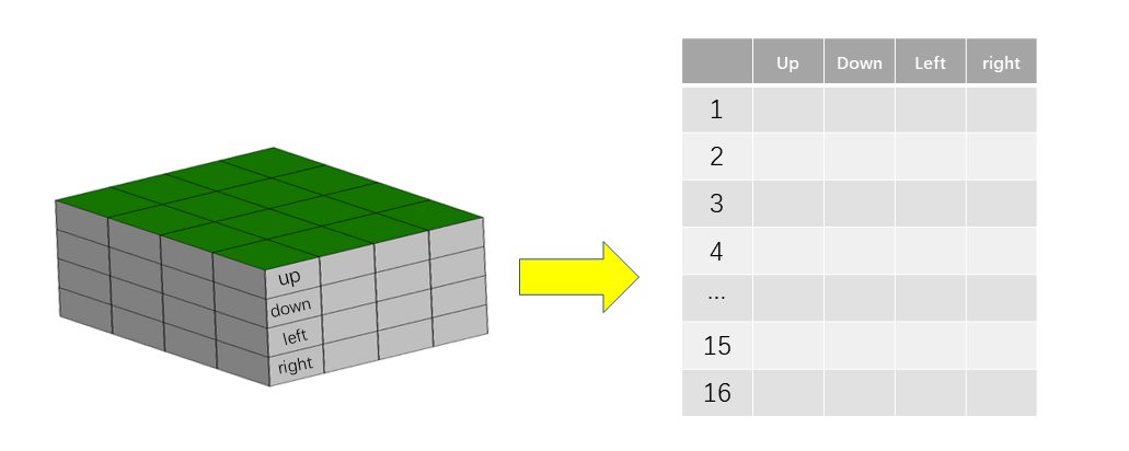
When initializing, we set each Q value in the Q-Table to 0. Now, directly use DataFrame in Pandas to output the Q-Table in the initial state:
def init_q_table():
    # Q-Table 初始化
    actions = np.array(["up", "down", "left", "right"])
    q_table = pd.DataFrame(
        np.zeros((16, len(actions))), columns=actions
    )  # 初始化 Q-Table 全为 0
    return q_table


init_q_table()
| up | down | left | right | |
|---|---|---|---|---|
| 0 | 0.0 | 0.0 | 0.0 | 0.0 |
| 1 | 0.0 | 0.0 | 0.0 | 0.0 |
| 2 | 0.0 | 0.0 | 0.0 | 0.0 |
| 3 | 0.0 | 0.0 | 0.0 | 0.0 |
| 4 | 0.0 | 0.0 | 0.0 | 0.0 |
| 5 | 0.0 | 0.0 | 0.0 | 0.0 |
| 6 | 0.0 | 0.0 | 0.0 | 0.0 |
| 7 | 0.0 | 0.0 | 0.0 | 0.0 |
| 8 | 0.0 | 0.0 | 0.0 | 0.0 |
| 9 | 0.0 | 0.0 | 0.0 | 0.0 |
| 10 | 0.0 | 0.0 | 0.0 | 0.0 |
| 11 | 0.0 | 0.0 | 0.0 | 0.0 |
| 12 | 0.0 | 0.0 | 0.0 | 0.0 |
| 13 | 0.0 | 0.0 | 0.0 | 0.0 |
| 14 | 0.0 | 0.0 | 0.0 | 0.0 |
| 15 | 0.0 | 0.0 | 0.0 | 0.0 |
86.9. Action Behavior Selection#
After obtaining the Q-Table, how to determine the next action strategy based on the Q-Table?
According to common sense, it is surely to choose the optimal decision (the action with the largest Q value) to maximize the long-term reward. However, some problems will arise, namely: in the initial learning, since the values in the Q-Table are random, they are meaningless for learning and prone to errors. After learning for a period of time, due to the fixed table values, each route will be fixed every time, and it is impossible to effectively explore the environment, easily falling into the local optimum problem.
So how should action selection be carried out?
The \(\varepsilon -greedy\) algorithm provides a good solution. Briefly speaking, when choosing an action, a probability value is introduced. With a certain probability, the optimal strategy is used for selection, and with a certain probability, a random selection is made. In this way, while trying to choose the optimal decision, exploration of the environment can be achieved.
Next, implement the function for action selection:
def act_choose(state, q_table, epsilon):
    """
    参数:
    state -- 状态
    q_table -- Q-Table
    epsilon -- 概率值

    返回:
    action --下一步动作
    """
    state_act = q_table.iloc[state, :]
    actions = np.array(["up", "down", "left", "right"])

    if np.random.uniform() > epsilon or state_act.all() == 0:
        action = np.random.choice(actions)
    else:
        action = state_act.idxmax()
    return action
86.10. Action Feedback Reward#
After the Agent little lion executes each action and immediately enters the next state, it will receive a reward from the environment to help itself learn.
Here, we set the reward value at the end point in the environment to 10 and the reward value at the trap to -10. At the same time, to help the model converge quickly, that is, to let the little lion find the shortest path as soon as possible, we set the reward value for each step to -1. This is also a small trick that penalizes the Agent for taking longer routes and spinning around in a certain area.
Next, write the feedback function for the Agent:
def env_feedback(state, action, hole, terminal):
    """
    参数:
    state -- 状态
    action -- 动作
    hole -- 陷阱位置
    terminal -- 终点位置

    返回:
    next_state -- 下一状态
    reward -- 奖励
    end --结束标签
    """
    # 行为反馈
    reward = 0.0
    end = 0
    a, b = state
    if action == "up":
        a -= 1
        if a < 0:
            a = 0
        next_state = (a, b)
    elif action == "down":
        a += 1
        if a >= 4:
            a = 3
        next_state = (a, b)
    elif action == "left":
        b -= 1
        if b < 0:
            b = 0
        next_state = (a, b)
    elif action == "right":
        b += 1
        if b >= 4:
            b = 3
        next_state = (a, b)

    if next_state == terminal:
        reward = 10.0
        end = 2
    elif next_state == hole:
        reward = -10.0
        end = 1
    else:
        reward = -1.0
    return next_state, reward, end
86.11. Q-Table Update#
Some basic elements of reinforcement learning have been constructed above. Next, we are going to let the Agent start learning. In this experiment, we use the Q-Learning algorithm, and the core of the Q-Learning algorithm lies in the update process of the Q-Table.
Q-Learning adopts the idea of the Bellman Equation for the update process of the Q-Table. Since the derivation of the Bellman Equation is complex, it will not be elaborated here. Students who are interested can view it through the link. Below, we will explain the update of the Q-Table in detail based on the example of the little lion walking through the maze.
Suppose the little lion reaches the upper-right grid. Define the state at this time as \(s_{t}\), the moving direction as \(a_{t}\), and the reward value Q for taking an action in the current state in the Q-Table is denoted as \(Q(s_{t},a_{t})\). After defining the basic variables, the formula for updating the Q value is directly given as follows:
It can be seen from the above formula that the update process of the Q value is actually a recursive iteration process.
Generally speaking, the update of the Q value mainly consists of two parts: the current reward value and the learning reward value, which are connected by the learning rate \(\alpha\). When the value of \(\alpha\) is higher, it means that less of the original value is retained and more importance is attached to the learning reward value, and vice versa.
The current reward value is the original value in the Q-Table, and the learning reward value also consists of two parts: \(r_{t + 1}\) (the reward after moving) and the estimation of the future optimal value. Here, the discount factor is introduced. Like a weight value, its role is to reduce the current reward for the estimated state in the future.
Since it is a recursive iteration process, we expand the recursive formula to gain a deeper understanding of the role of the discount factor. For the convenience of writing, we abbreviate the formula here. Assume that \(Q(s_{1})\) is the reward value in the initial state. Then the update formula for \(Q(s_{1})\) is:
Expand equation \((1)\):
Among them, \(\gamma\) is a number between 0 and 1. Through power calculation, it can be easily found that the later the reward, the smaller the impact on the current estimated value.
Next, we implement the function for Q-Table update:
def update_q_table(q_table, state, action, next_state, terminal, gamma, alpha, reward):
    """
    参数:
    q_table -- Q-Table
    state -- 状态
    action -- 动作
    next_state -- 下一状态
    terminal -- 终点位置
    gamma -- 折损因子
    alpha -- 学习率
    reward -- 奖励

    返回:
    q_table -- 更新后的Q-Table
    """
    # Q-Table 的更新函数
    x, y = state
    next_x, next_y = next_state
    q_original = q_table.loc[x * 4 + y, action]
    if next_state != terminal:
        q_predict = reward + gamma * q_table.iloc[next_x * 4 + next_y].max()
    else:
        q_predict = reward
    q_table.loc[x * 4 + y, action] = (1 - alpha) * q_original + alpha * q_predict
    return q_table
To facilitate observing the process of the little lion’s step-by-step training to find the big ham, we define an auxiliary function below. This function is convenient for visualizing the state of the little lion at each step.
def show_state(end, state, episode, step, q_table):
    """
    参数:
    end -- 结束标签
    state -- 状态
    episode -- 迭代次数
    step --迭代步数
    q_table-- Q-Table
    """
    # 状态可视化辅助函数
    terminal = (3, 2)
    hole = (2, 1)
    env = np.array([["_ "] * 4] * 4)
    env[terminal] = "$ "
    env[hole] = "# "
    env[state] = "L "
    interaction = ""
    for i in env:
        interaction += "".join(i) + "\n"

    if state == terminal:
        message = "EPISODE: {}, STEP: {}".format(episode, step)
        interaction += message
        display.clear_output(wait=True)  # 清除输出内容
        print(interaction)
        print("\n" + "q_table:")
        print(q_table)
        time.sleep(3)  # 在成功到终点时,等待 3 秒
    else:
        display.clear_output(wait=True)
        print(interaction)
        print(q_table)
        time.sleep(0.3)  # 在这里控制每走一步所需要时间
After defining the visualization function, next, we implement Q-Learning according to the Q-Learning algorithm process. The following gives the pseudocode and explanations of the Q-Learning algorithm:
Initialize Q arbitrarily // Initialize Q values randomly
Repeat (for each episode): // Each game is called an episode
    Initialize S // The state of the little lion's initial position
    Repeat (for each step of episode):
        Based on the current Q and position S, use the ε-greedy strategy to obtain action A
        After taking action A, the little lion reaches a new position S' and receives a reward R
        Q(S,A) ← (1-α)*Q(S,A) + α*[R + γ*maxQ(S',a)] // Update S in Q
        S ← S'
    until S is terminal // The little lion finds the big ham or falls into a trap and starts over
The update formula of the Q-Table in the pseudocode is only different in the form of expression from the update formula of the Q-Table described in 3.5, but they have the same practical meaning.
Next, the complete implementation function of the Q-Learning algorithm is given:
def q_learning(max_episodes, alpha, gamma, epsilon):
    """
    参数:
    max_episodes -- 最大迭代次数
    alpha -- 学习率
    gamma -- 折损因子
    epsilon -- 概率值

    返回:
    q_table -- 更新后的Q-Table
    """
    q_table = init_q_table()
    terminal = (3, 2)
    hole = (2, 1)
    episodes = 0
    while episodes <= max_episodes:
        step = 0
        state = (0, 0)
        end = 0
        show_state(end, state, episodes, step, q_table)
        while end == 0:
            x, y = state
            act = act_choose(x * 4 + y, q_table, epsilon)  # 动作选择
            next_state, reward, end = env_feedback(state, act, hole, terminal)  # 环境反馈
            q_table = update_q_table(
                q_table, state, act, next_state, terminal, gamma, alpha, reward
            )  # q-table 更新
            state = next_state
            step += 1
            show_state(end, state, episodes, step, q_table)
        if end == 2:
            episodes += 1
Now we have finally implemented the entire Q-Learning algorithm, which can help the little lion find the big ham. Next, we specify the parameters and execute the function to observe how the little lion uses the Q-Learning algorithm to find the shortest path to the big ham placement point.
q_learning(max_episodes=10, alpha=0.8, gamma=0.9, epsilon=0.9)
_ _ _ _
_ _ _ _
_ # _ _
_ _ L _
EPISODE: 10, STEP: 5

q_table:
          up      down      left     right
0  -2.382398  3.094751 -2.213120 -2.284452
1  -2.213120 -2.134708 -2.238334 -1.804800
2  -1.536000 -1.568000 -2.230358 -1.651200
3  -1.536000 -0.998400 -1.683200 -1.536000
4  -0.302803  4.575375 -1.536000 -1.536000
5  -1.719450 -9.600000 -0.195464 -1.691187
6  -1.376000 -0.999680 -1.897574 -1.689600
7  -1.852160 -1.536000 -1.710848 -0.992000
8   0.695038  6.199484 -0.992000 -8.000000
9   0.000000  0.000000  0.000000  0.000000
10 -1.876736  0.000000 -8.000000 -0.992000
11 -1.536000  4.800000 -0.960000 -0.800000
12  0.630620  4.650713 -1.536000  7.999966
13 -8.000000  4.800000  3.297792  9.999999
14  0.000000  0.000000  0.000000  0.000000
15  2.656000  4.960000  8.000000  4.960000
By running the program, it can be very intuitive to see that as the number of iterations increases, the path taken by the little lion becomes more and more correct, and the number of STEPs used will also become less and less until the shortest path is found. However, after finding the shortest path, there may still be a situation where the number of STEPs increases. This is the result of introducing \(\varepsilon -greedy\) for random exploration, which is a very normal phenomenon.
86.12. Sarsa Learning Algorithm#
In value-based reinforcement learning algorithms, there is another algorithm similar to Q-Learning called Sarsa. Next, let’s briefly look at the differences between the Sarsa learning algorithm and the Q-Learning algorithm from the principles and algorithm processes.
Sarsa is essentially similar to Q-Learning. The biggest difference lies in the update of the Q-Table. Next, let’s first understand Sarsa from the pseudocode.
From the pseudocode, the algorithm process of Sarsa can be summarized into the following steps.
-
Initialize the Q-Table: Construct a table with the same dimensions according to the environment and action types. (Same as Q-Learning)
-
Action selection: Select the next action based on the values in the Q-Table. (Same as Q-Learning)
-
Action feedback: Obtain the action feedback given by the environment after taking an action. (Same as Q-Learning)
-
Q-Table update: Update the Q-Table according to the feedback and the actual reward of the next state. (Different from Q-Learning)
Repeat steps 2 to 4 until the expected result is achieved or the pre-set number of iterations ends. Then output the Q-Table to complete Sarsa.
You will find that, compared with the learning process of the Q-Learning algorithm, there is only one difference in the description of one of the steps in Sarsa. That is, in Q-Learning, we update the Q-Table according to the feedback and the estimated future reward. While in Sarsa, we update the Q-Table according to the feedback and the actual reward of the next state.
86.13. Differences between Sarsa and Q-Learning#
Regarding the differences between the Sarsa and Q-Learning algorithms, it is not intuitive to understand from either the pseudocode or the algorithm principle. Below, we will illustrate it vividly in the form of a diagram.
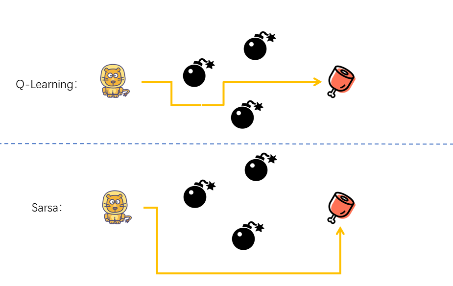
The Q-Learning algorithm is actually an Off-Policy algorithm, that is, it can learn through estimation or other predictions.
When updating the Q-Table, Q-Learning adopts a “greedy” algorithm, that is, it updates according to the estimated future reward value. Actually, it is manifested as: the little lion is very adventurous. When choosing a path, it gives top priority to finding the big ham. No matter how dangerous the journey is, as long as it can get closer to the big ham, it will move forward.
Compared with the “idealistic” algorithm of Q-Learning that updates the Q-Table through estimation, Sarsa is more “pragmatic”. It is an On-Policy algorithm, that is, it learns through the experience generated by its own experiences. And On-Policy means following the established policy. The difference between it and the Off-Policy Q-Learning algorithm is as follows, that is, whether the method used to update Q is to follow the established policy (on-policy) or use a new policy (off-policy).
Difference |
Q-Learning |
Sarsa |
|---|---|---|
|
Select the next action A’ |
ε-greedy policy |
ε-greedy policy |
Update the Q value |
greedy policy |
ε-greedy policy |
When updating the Q-Table, Sarsa uses actual actions for the update, that is, after entering \(S_{t + 1}\), it updates \(Q(S_{t}, a)\). Actually, it is manifested as: the little lion appears very cautious. When choosing a path, it pays more attention to the existence of traps and takes a detour to avoid the traps.
After completing the challenges of this experiment and through presenting the comparison, it will be found that using the Q-Learning algorithm is easier to find a suitable path than the Sarsa algorithm. However, during the process of finding a suitable path, the Q-Learning algorithm fails more times than the Sarsa algorithm.
In this experiment, we will not implement the Sarsa algorithm. You will try to implement the update process of the Sarsa algorithm by yourself in the following challenges.
86.14. Summary#
This experiment has provided a detailed introduction to value-based reinforcement learning algorithms. However, since the content of reinforcement learning is quite abstract, it requires everyone to study and train repeatedly.
Related Links