Pro Membership

Pro Membership is a membership plan created by the author to maintain and update this tutorial. You can get more benefits and services, click to view details.

62. Principles and Practices of Image Classification

62.1. Introduction

In this experiment, we will focus on the image classification problem in the engineering applications of machine learning. In previous experiments, we have actually learned to use simple convolutional neural networks to complete image classification. In fact, for some relatively complex datasets, simple convolutional neural networks cannot achieve a high classification accuracy, while the network structures in deep learning practice usually can reach dozens or even hundreds of layers. Therefore, in this experiment, we will use the classical network structures that have been repeatedly proven to be very powerful and use transfer learning to complete the relatively complex classification task of cat and dog recognition.

62.2. Key Points

• Data Loader

• Transfer Learning

• Cat and Dog Recognition

• Visualization of Convolutional Neural Networks

Computer vision is a science that studies how to enable machines to “see”, encompassing a variety of key technologies and application scenarios. With the rapid development of deep learning, computer vision has also迎来了新的发展趋势。Currently, deep learning is mainly good at doing the following in computer vision: image classification, object detection, target tracking, semantic segmentation, and instance segmentation. （注：原文中“迎来了新的发展趋势”表述不太完整准确，这里按字面翻译了。）

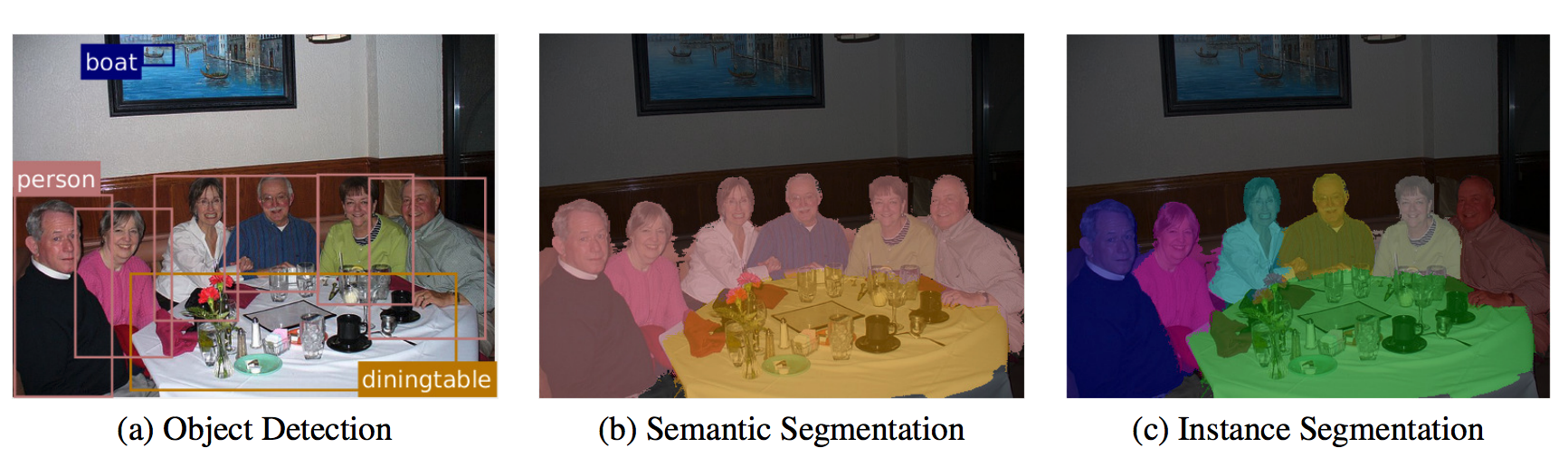
Image Classification, is one of the most representative practical scenarios in which deep learning is applied to computer vision. As the name implies, image classification is easy to understand and can be applied to practical tasks such as image retrieval. Object Detection means detecting key objects in an image. In object detection tasks, we usually use bounding boxes to enclose the detected objects and mark the confidence levels. Object Tracking refers to the process of tracking one or more specific objects of interest in a specific scenario and is one of the key technologies for autonomous driving. Semantic Segmentation can be regarded as an extension of object detection, which not only requires marking the bounding boxes of the objects but also accurately identifying the boundaries of each part.

Finally, Instance Segmentation is an extension of Semantic Segmentation. For example, different instances of objects in the same category are marked with specific colors.

Source

Next, we will try to understand the application of image classification and learn to build an excellent image classifier using the method of transfer learning.

62.3. Dataset

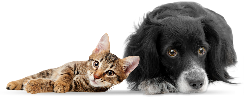
In this experiment, we will solve the famous “Cat and Dog Recognition” image classification problem. “Cat and Dog Recognition” is a popular image classification competition on Kaggle. The training set contains a total of 25,000 labeled cat and dog photos, with an equal number of cats and dogs. The test set has 12,500 photos, which are not labeled as cats or dogs and are the prediction results that need to be submitted for the competition.

{note}
This experiment requires a GPU to run properly. You can select a GPU instance with at least NVIDIA Tesla T4 in Colab.

In this experiment, we only download the labeled training set. And in the following experiments, we will divide this dataset into a training set and a validation set at a ratio of 4:1. Here, we call it the validation set to distinguish it from the original test set provided by Kaggle.

Next, the experiment downloads the labeled training data [543 MB] provided in the “Cat and Dog Recognition” challenge.

wget -nc 'http://labfile.oss.aliyuncs.com/courses/1081/dogs_cats.zip'  # 下载数据
unzip -o "dogs_cats.zip"  # 解压数据

In the dataset, the images are named in the format of type.num.jpg, which represent the label and the sample number respectively. For example: cat.9586.jpg or dog.1328.jpg, etc.

Next, traverse the file directory to load the dataset:

import os

data_path = []
data_name = []

for root, dirs, files in os.walk("train"):
    # 变量指定目录文件列表
    for image_file in files:
        image_path = os.path.join(root, image_file)
        data_path.append(image_path)
        data_name.append(image_file.split(".")[0])

len(data_path), len(data_name)

(25000, 25000)

In this process, first, we read the paths of each photo and save them to the list data_path, and then obtain the corresponding labels by splitting the file names.

Let’s randomly select sixteen images to see what the samples in the cat and dog dataset look like specifically. Here we use the conversion and display methods provided by the torchvision tool.

pip install -U scikit-image  # 安装 scikit-image

import random
from torchvision.utils import make_grid
from torchvision import transforms
from skimage import io, transform
import matplotlib.pyplot as plt

%matplotlib inline

# 随机抽取 16 张图片路径
img_path_list = random.sample(data_path, 16)
# 使用 skimage 根据路径读取图片并对显示尺寸进行裁剪
img_list = [
    transform.resize(io.imread(img_path), (100, 100), mode="reflect")
    for img_path in img_path_list
]
# 使用 torchvision 将图片处理成张量
img_list = [transforms.ToTensor()(img) for img in img_list]
# 将图片合并成每行四张的大图
img_show = make_grid(img_list, nrow=4, normalize=True)
plt.figure(figsize=(6, 6))
plt.imshow(img_show.permute(1, 2, 0).numpy())

<matplotlib.image.AxesImage at 0x7f4cbc01f580>

After looking at the images in the cat and dog dataset, we generally understand what the dataset looks like. Next, we need to preprocess the labels. After all, during training, we cannot directly accept string data, but only numerical labels.

Different from the previous operations, at this time, we can use sklearn.preprocessing.LabelEncoder 🔗 to standardize the labels, converting string labels into numerical labels starting from 0. Additionally, this method can also reverse the labels, that is, convert numbers into strings. Of course, you can also write a conditional statement by yourself to numericalize the string labels.

from sklearn.preprocessing import LabelEncoder

le = LabelEncoder()
le.fit(["cat", "dog"])
data_label = le.transform(data_name)
data_label

array([0, 1, 0, ..., 1, 0, 1])

Compared with the character labels, you should be able to find that here, cats and dogs are replaced with 0 and 1 respectively.

62.4. Data Loader

Above, we have roughly completed two data preparation tasks. First, we have read the image paths, but have not yet processed the images into tensors that can be input into the network. Second, we have converted the image labels into a usable type. Therefore, next, we will use a series of methods provided by PyTorch to create an image data loader.

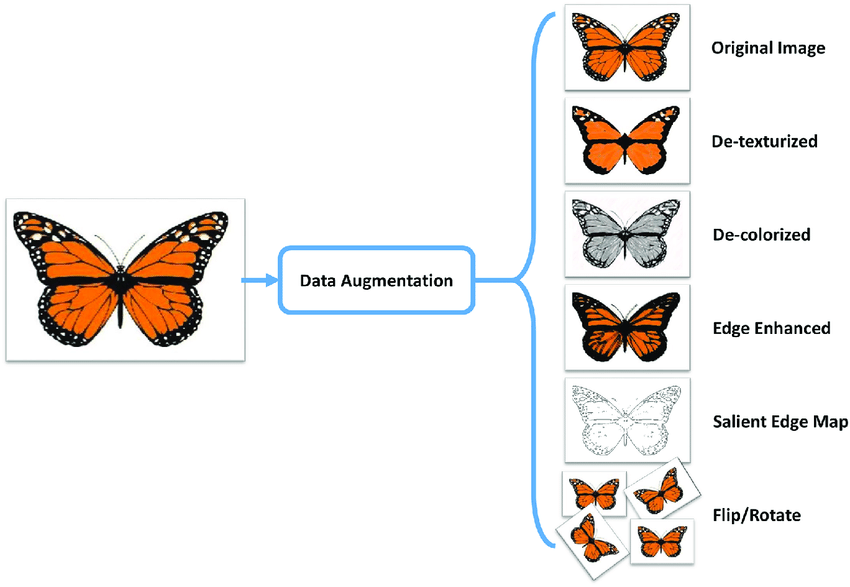
Before officially creating a PyTorch data loader, we need to first understand a concept called Data Augmentation. Simply put, the performance of deep learning highly depends on the scale of the dataset. Naturally, we hope for a dataset of sufficient size. However, in many cases, due to various constraints, the dataset may not be large enough. Then, for image data, operations such as random cropping, rotation, mirroring, and desaturation can be used to transform a single image into multiple images with different perspectives and angles, achieving the effect of data augmentation. In addition, generating new images through the GAN learned previously is also a way of data augmentation.

Source

torchvision.transforms provided by PyTorch 🔗 has built-in many image processing functions, and by reasonable combination, the effect of data augmentation can be achieved.

Let’s take a look at the processing operations to be used here:

import numpy as np

# 加载图片并转换为 PIL IMAGE
IMAGE = transforms.ToPILImage()(io.imread(data_path[0]))
# 尺寸变形
scale = transforms.Resize(256)
# 随机裁剪
crop = transforms.RandomCrop(128)
# 打包方法
composed = transforms.Compose([transforms.Resize(256), transforms.RandomCrop(224)])
# 将每个变换函数应用到一个样本上
fig = plt.figure()
for i, tsfrm in enumerate([scale, crop, composed]):
    transformed_sample = np.array(tsfrm(IMAGE))  # PIL.image 转换成 np.ndarray
    ax = plt.subplot(1, 3, i + 1)
    plt.tight_layout()
    ax.set_title(type(tsfrm).__name__)
    ax.imshow(transformed_sample)

In the above example, ToTensor converts a PIL Image or a numpy.ndarray into a Tensor type in PyTorch. The data format of a PIL Image and a numpy.ndarray is height \(\times\) width \(\times\) channel, and the pixel range is in \([0, 255]\). The converted Tensor is channel \(\times\) height \(\times\) width, and the range is between \([0.0, 1.0]\).

The three images finally returned are, in sequence: resized only using Resize, randomly cropped only using RandomCrop, and processed using the combined method of Resize and RandomCrop.

Next, let’s define the transforms preprocessing operations required for the data loader.

data_transforms = {
    "train": transforms.Compose(
        [
            transforms.ToPILImage(),
            transforms.Resize(256),
            transforms.RandomCrop(224),
            transforms.RandomHorizontalFlip(),  # 水平镜像
            transforms.ToTensor(),
            transforms.Normalize(
                [0.485, 0.456, 0.406], [0.229, 0.224, 0.225]  # 用平均值和标准偏差归一化张量图像
            ),  # input = (input - mean) / std
        ]
    ),
    "val": transforms.Compose(
        [
            transforms.ToPILImage(),
            transforms.Resize(256),
            transforms.CenterCrop(224),  # 测试只需要从中间裁剪
            transforms.ToTensor(),
            transforms.Normalize(
                [0.485, 0.456, 0.406], [0.229, 0.224, 0.225]  # mean
            ),  # std
        ]
    ),
}

Among them, data augmentation and data normalization are required for training. For validation data, it only needs to be cropped to the size of the training data without augmentation, because this can ensure the accuracy of evaluation.

After defining the preprocessing operations, next, first split the data into a training set and a validation set in a ratio of 4:1, directly using the familiar train_test_split function.

from sklearn.model_selection import train_test_split

train_path, val_path, train_label, val_label = train_test_split(
    data_path, data_label, test_size=0.2
)

len(train_path), len(val_path), len(train_label), len(val_label)

(20000, 5000, 20000, 5000)

Remember the torchvision.datasets.ImageFolder 🔗 used when creating the data loader in the “Generate Anime Character Avatars” experiment? This method can directly read a custom image folder, which is very convenient and useful. Unfortunately, this method cannot be used to load cat and dog recognition images here. The reason is that the API of torchvision.datasets.ImageFolder 🔗 requires the images to be stored in the following format:

train/dog/xxx.jpg
train/dog/xxy.jpg
train/dog/xxz.jpg

train/cat/123.jpg
train/cat/nsdf3.jpg
train/cat/asd932_.jpg

That is to say, you need to store the pictures of different categories in separate subfolders according to their categories. However, in the data we provided, all the pictures are in one folder.

Next, following the idea provided in the PyTorch official tutorial, we adapt the image data in any organizational form by inheriting and overriding the torch.utils.data.Dataset 🔗 class. I hope this will inspire you in the actual data loading process later.

torch.utils.data.Dataset is an abstract class. When customizing a Dataset, you must inherit from torch.utils.data.Dataset and then override the following methods:

• __len__: Returns the size of the dataset.

• __getitem__: Reads and returns the data by index.

In __init__, variables can be initialized or operations that are only done once can be performed, such as reading the label file, etc. While in __getitem__, it is used to read the images and return the image data and labels.

from torch.utils.data import Dataset


class DogcatDataset(Dataset):
    def __init__(self, data_path, data_label, transform=None):
        """
        - data_path (string): 图片路径
        - data_label (string): 图片标签
        - transform (callable, optional): 作用在每个样本上的预处理函数
        """
        self.data_path = data_path
        self.data_label = data_label
        self.transform = transform

    def __len__(self):
        return len(self.data_path)

    def __getitem__(self, idx):
        img_path = self.data_path[idx]
        image = io.imread(img_path)
        label = self.data_label[idx]

        # 如果有，则对数据预处理
        if self.transform:
            image = self.transform(image)

        return image, label

Next, initialize the two Datasets for training and testing respectively:

# 初始化训练数据集
train_dataset = DogcatDataset(train_path, train_label, data_transforms["train"])
# 初始化测试数据集
val_dataset = DogcatDataset(val_path, val_label, data_transforms["val"])
train_dataset, val_dataset

(<__main__.DogcatDataset at 0x7f4cb90bfac0>,
 <__main__.DogcatDataset at 0x7f4cb90bfc10>)

The Dataset class can be loaded using a for i in range loop iteration. However, in actual development, the more advanced torch.utils.data.DataLoader is usually used for iteration because it supports mini-batch loading, shuffling the data, and multi-threaded reading features. This method has also been learned in the previous experiments.

import torch

# 训练数据加载器
train_loader = torch.utils.data.DataLoader(train_dataset, batch_size=64, shuffle=True)
# 验证数据加载器
val_loader = torch.utils.data.DataLoader(val_dataset, batch_size=64, shuffle=False)

train_loader, val_loader

(<torch.utils.data.dataloader.DataLoader at 0x7f4cb90bf0d0>,
 <torch.utils.data.dataloader.DataLoader at 0x7f4cb90bf730>)

So far, we have importantly completed the creation of the data loader. You may find that this process is more complex than you might imagine. In fact, since most of the previous experiments used the built-in datasets provided by the framework for practice, it has helped us skip a large number of intermediate processes. In real application scenarios, preprocessing and loading data is a rather troublesome task.

Next, use the data loader to load a mini-batch to verify whether it can work properly.

for batch_index, sample_batch in enumerate(train_loader):
    images, labels = sample_batch
    sample_images = make_grid(images, normalize=True)
    plt.figure(figsize=(8, 8))
    plt.imshow(sample_images.permute(1, 2, 0).numpy())
    break

With the data loader, can we start building a neural network for the cat and dog recognition task?

Sure. However, for those without an academic background, customizing a convolutional neural network structure can be used to complete simple image classification tasks like MNIST, but it is very difficult for problems like cat and dog recognition. Because you lack experience.

So, generally speaking. Engineers should try their best to use the relatively classic neural network structures mentioned in our convolutional neural network principle experiments, rather than designing them by themselves. For example: AlexNet, VGG, Google Net, and ResNet, etc.

In this experiment, we first choose the relatively simple AlexNet network structure. However, we still won’t build an AlexNet from scratch using PyTorch by ourselves. The reason is that although data augmentation has been performed, the cat and dog recognition dataset is still relatively small. At the same time, it takes a very long time to train an AlexNet from scratch, which ranges from several hours to more than a dozen hours.

Therefore, this experiment will introduce you to a new learning method: transfer learning. Transfer learning can not only shorten the training time, but also often achieve much better results than training from scratch. Next, let’s learn this method that kills two birds with one stone.

62.5. Overview of Transfer Learning

Let’s use an intuitive example to illustrate what transfer learning is. Suppose you travel back in time to ancient times and become the crown prince. To govern the country well, you need to know so much. If you start learning from scratch, it will definitely be too late. What you need to do is to find your emperor father and ask him what he is doing, and he also hopes to transfer all the knowledge in his mind to yours at once.

This is exactly transfer learning, which is to learn knowledge or experience from previous tasks and apply it to new tasks. In other words, the purpose of transfer learning is to extract knowledge and experience from one or more source tasks and then apply it to a target domain. For example, a general speech model is transferred to a person’s speech recognition, and a pre-trained image classification model is transferred to medical disease recognition.

What was said above sounds very simple, but in terms of neural networks, it means that the weights of each node in each layer of the network are transferred from a trained network to a brand-new network. Instead of starting from scratch and training a neural network for each specific task.

The benefits of doing this can be demonstrated by the following example. Suppose there is already a deep neural network that can accurately distinguish between cats and dogs. Later, if you want to train a model that can distinguish pictures of different breeds of dogs, what you need to do is not to train the first few layers of the neural network that are used to distinguish straight lines and acute angles from scratch. Instead, use the trained network to extract the primary features, and then only train the last few layers of neurons so that they can distinguish the breeds of dogs.

Source

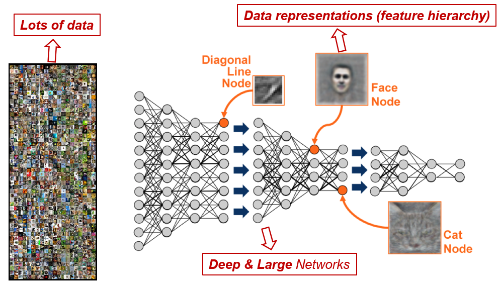
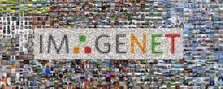
In fact, very few people train the entire convolutional network from scratch (random initialization) because having a dataset of sufficient size is relatively rare. Instead, ConvNets are usually pre-trained on very large datasets and then used as an initialization or fixed feature extractor for the task of interest. Among them, ImageNet is a commonly used large-scale dataset, which contains more than 14 million images with 20,000 categories 🔗. Most of the papers on the classical convolutional neural networks mentioned above use the evaluation results on ImageNet.

Source

Transfer learning is widely applied, especially in the engineering field, whether it is dealing with accents in different regions in speech recognition or training autonomous vehicles through the simulated images of video games in the early stage. At the same time, transfer learning is also a research hotspot in the academic community, which mainly focuses on the following aspects:

• Reduce the dependence on labeled data through semi-supervised learning to address the asymmetry of labeled data.

• Improve the stability and generalization ability of the model through transfer learning so that the classification result will not change due to the change of a single pixel.

• Use transfer learning to achieve continuous learning, enabling the neural network to retain the skills learned in old tasks.

62.6. Transfer Learning Strategies

According to the different characteristics of transfer learning, generally speaking, there are the following three different learning strategies for transfer learning. The boundaries of these strategies are not particularly obvious, and there are connections among them.

62.6.1. Pre-trained Models

ImageNet has tens of millions of images, and current convolutional neural networks are quite complex with a very large number of training parameters. Therefore, even when training on many GPUs, it takes 2 to 3 weeks. So, in order to release the model, the trained model parameters are often saved for others to fine-tune using this model. Many deep learning frameworks provide pre-trained models. For example, the earliest Caffe opened a large number of pre-trained models in Model Zoo. These models can be directly used.

62.6.2. Feature Extractor

Pre-train a convolutional network ConvNet on ImageNet, remove the last fully connected layer (the output of this layer is the probabilities of a sample in ImageNet corresponding to 1000 classes), and then regard the remaining ConvNet as a fixed feature extractor for the new dataset. Then train a linear classifier (such as a linear SVM or Softmax classifier) for the new dataset. For example, in the cat and dog classification, there are 2 classes, namely cats and dogs, and only the last layer needs to be trained to achieve binary classification.

62.6.3. Fine-tuning

This strategy is not only to replace and retrain the classifier on top of the ConvNet on the new dataset, but also to fine-tune the weights of the pre-trained network by continuing backpropagation, and all layers of the ConvNet can be fine-tuned. Of course, due to the overfitting problem, some early layers can also be retained and only some higher-level parts of the network can be fine-tuned.

The characteristics of ordinary pre-trained models are that they are trained with large datasets and already have the ability to extract shallow basic features and deep abstract features. Then, when no fine-tuning is done, the following situations are likely to occur:

• Training from scratch requires a large amount of data, computing time, and computing resources.

• There are risks such as the model not converging, the parameters not being optimized enough, low accuracy, low model generalization ability, and being prone to overfitting.

Using fine-tuning can effectively avoid the above possible problems. Generally, when encountering the following situations during parameter tuning, fine-tuning will be considered:

• The dataset used is similar to the dataset of the pre-trained model. If they are not very similar, for example, if the pre-trained parameters are for natural scenery pictures but you want to do face recognition, the effect may not be so good because the feature extraction of faces and natural scenery is different, so the corresponding parameters are also different after training.

• The accuracy of the convolutional neural network model built or used by yourself is too low. You can try fine-tuning to see if it can improve the performance of your network.

• The datasets are similar, but the number of datasets is too small.

• The computing resources are too scarce.

So, how should we perform the fine-tuning operation? We can start from the following aspects:

• The common approach is to truncate the last layer (classifier) of the pre-trained network and replace it with a new classifier. For example, a network pre-trained on ImageNet comes with a Softmax layer for 1000 classes. If the new task is to classify 10 classes, the new Softmax layer of the network will consist of 10 classes instead of 1000. Then run the pre-trained weights on the network. Make sure to perform cross-validation so that the network can generalize well.

• Use a smaller learning rate to train the network. Since the pre-trained weights are already quite good compared to randomly initialized weights, these weights are generally not changed too quickly. So, the initial learning rate commonly used is 1/10 of the initial learning rate for training from scratch.

• If the number of datasets is too small, generally only train the last layer. If the number of datasets is moderate, you can freeze the first few layers of the pre-trained network and train the last few layers. Because the first few layers capture general features relevant to the new problem, such as curves and edges, and we want to keep these weights unchanged. Instead, generally let the network focus on learning dataset-specific features in the subsequent deeper layers.

62.7. Overfitting and Underfitting

Before formally conducting transfer learning, let’s take a closer look at the concepts of overfitting and underfitting. An important topic in machine learning is the “generalization ability” of the model. A model with strong generalization ability is a good model. For a trained model, if its performance on the training set is poor, it goes without saying that its performance on the test set will also be very poor, which may be caused by underfitting; if the model performs very well on the training set but is mediocre on the test set, then this is caused by overfitting.

In machine learning, the error that a model shows on the training dataset is called the training error, and the expected value of the error shown on any test data sample is called the generalization error.

The performances of underfitting and overfitting in terms of error are as follows:

• Underfitting: The machine learning model cannot achieve a low training error.

• Overfitting: The training error of the machine learning model is much smaller than its error on the test dataset.

Source

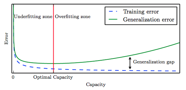
As shown in the figure above, the first half of the red line represents underfitting, where the generalization error fails to converge (decrease). The second half of the red line represents overfitting. The training error of the network is decreasing, but the generalization error keeps increasing and is higher than the training error.

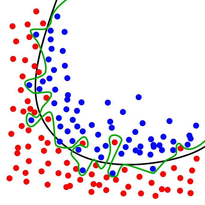
For example, use a curve to separate many points on a plane. The red and green dots correspond to the training set. The green line represents an overfitting model, and the black line represents a regularized model. Although the error of the green line on the training data is very small, it is too dependent on that data. In other words, the green line overfits the data. So compared with the black line, the green line may have a higher error on newly added data, which corresponds to the test set.

Source

If the model fails to consider enough information to accurately model the real world, the phenomenon of underfitting will occur. For example, if only two points on the exponential curve in the following figure are observed, it may be asserted that there is a linear relationship here. However, it is also possible that there is no pattern at all because only two points are available for reference. In the interval \([-1, +1]\), a straight line can provide a good approximation of the exponential curve:

Source

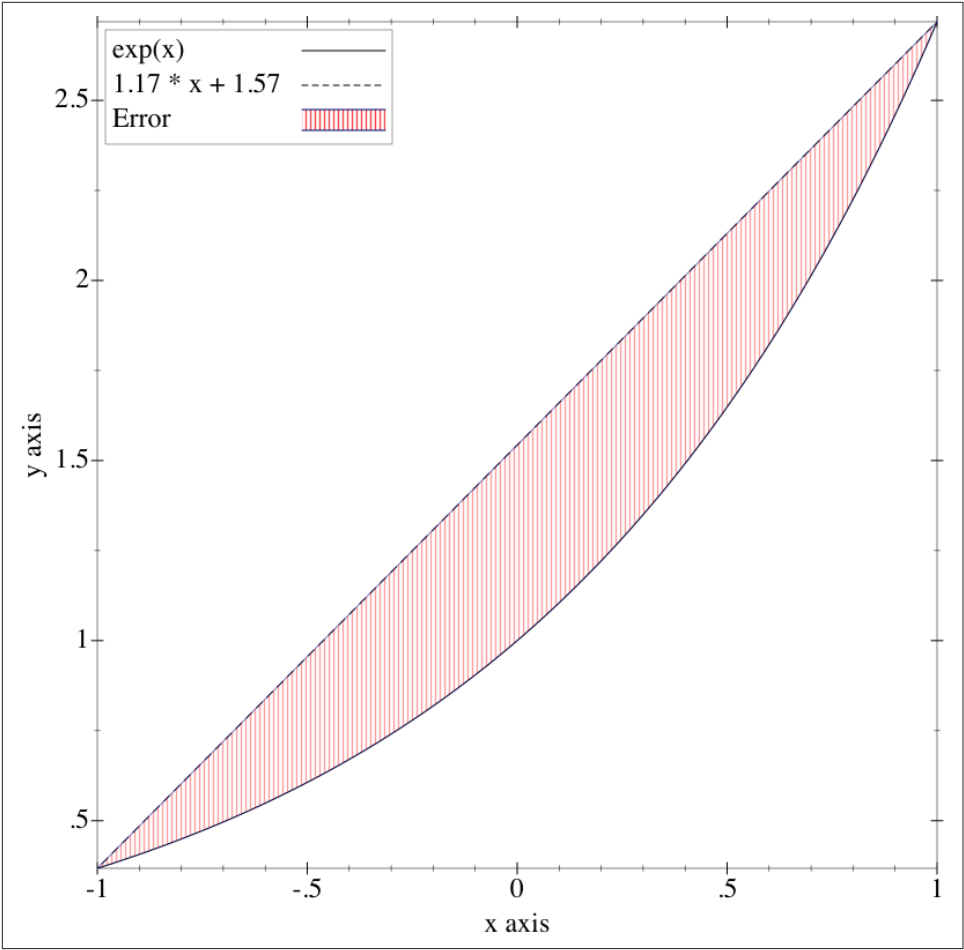
However, in the interval \([-20, 20]\), the straight line not only fails to fit the exponential curve, but also has a very large error. Since the ordinate values are very large at this time, the function graph represented by the dotted line is already close to the X-axis.

Source

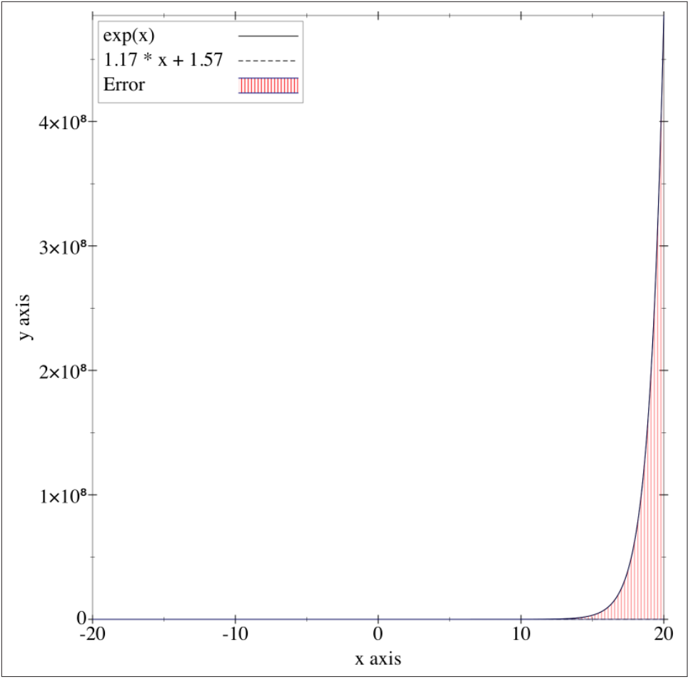
This is overfitting. Due to a lack of samples or too few features being set, the model fails to obtain sufficient information and thus cannot arrive at a good solution.

Generally, when we encounter overfitting, there are mainly the following solutions:

• Clean the data again. One possible reason for overfitting is impure data, which requires us to clean the data again.

• Insufficient training data volume. In this case, we can increase the proportion of training data in the total data or perform data augmentation, such as inverting, mirroring, and cropping images.

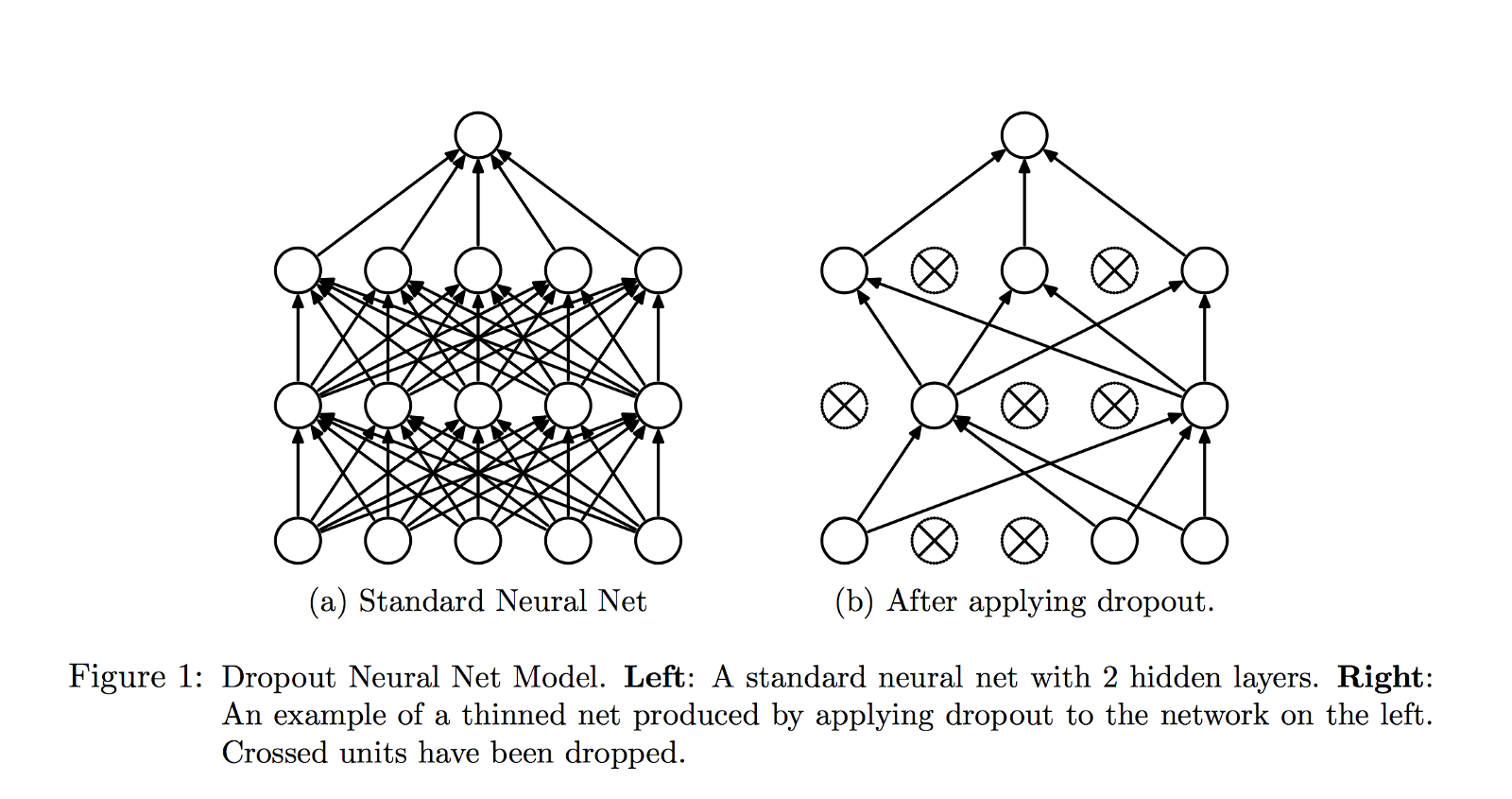
• Adopt the Dropout method. Dropout is a regularization method for neural networks that disconnects neurons with a certain probability during training.

• Batch normalization. As the name implies, Batch normalization normalizes each batch of data. Its main function is to accelerate the training speed of the network, but to some extent, it also replaces the role of Dropout. Batch normalization introduces randomness during the training phase to prevent overfitting. During the testing phase, this randomness is removed globally by taking the expectation and other means to obtain definite and accurate results.

• Add L1/L2 regularization terms. This method can be directly achieved by adding penalty terms to the training parameters.

Correspondingly, there are far fewer solutions to underfitting. Underfitting is mainly caused by the network not learning sufficiently, so it can be improved by optimizing the network structure. Generally, the number of features extracted can be increased by adding more network layers. For example, replacing AlexNet with ResNet.

Source

Additionally, if the learning rate is not appropriately selected, it may also exhibit characteristics of underfitting and overfitting. However, in fact, this is not caused by underfitting or overfitting, which can be specifically described as:

• Loss jitter: The overshoot phenomenon caused by too large a learning rate, that is, continuously diverging at both ends of the extreme point, or oscillating violently. In short, as the number of iterations increases, there is no tendency for Loss to decrease.

• Slow Loss decrease: This is the reason why the learning rate is too small, resulting in the convolutional neural network learning too slowly.

• Loss explosion, even exceeding the range of real number representation: The learning rate is extremely large, and the optimizer simply cannot work properly.

Generally, some learning rate decay strategies are selected to avoid the above problems encountered with a fixed learning rate:

• Step decay: Reduce the learning rate every certain number of training epochs. Usually, a fixed value is given, for example, 0.1 times the previous learning rate.

• Exponential decay: Decay according to the formula \(\alpha = \alpha_0 e^{-k t}\), where \(\alpha_0\) and \(k\) are hyperparameters, and \(t\) is the number of iterations.

• 1/t decay: Decay according to the formula \(\alpha = \alpha_0 \div (1 + k t )\), where \(\alpha_0\) and \(k\) are hyperparameters, and \(t\) is the number of iterations.

For the learning rate decay scheme, most deep learning frameworks provide corresponding parameters for adjustment.

62.8. Transfer Learning for Cat and Dog Recognition

Fine-tuning in transfer learning is relatively simple. One only needs to load the weights of the pre-trained model, then change the number of outputs of the classifier and retrain. However, this method takes a relatively long time.

Therefore, here we will introduce the second method, which uses the pre-trained model as a fixed feature extractor and only trains the last layer classifier. In this experiment, we will use the pre-trained AlexNet model. We directly load the AlexNet model pre-trained on ImageNet from PyTorch. 🔗

Pre-trained model [240MB] takes time to download. If the progress is extremely slow, you can forcefully abort and re-execute the download.

from torchvision import models

# 从课程镜像服务器上下载 AlexNet 预训练模型
torch.utils.model_zoo.load_url(
    "https://cdn.aibydoing.com/aibydoing/files/alexnet-owt-4df8aa71.pth"
)
alexnet = models.alexnet(pretrained=True)
alexnet

AlexNet(
  (features): Sequential(
    (0): Conv2d(3, 64, kernel_size=(11, 11), stride=(4, 4), padding=(2, 2))
    (1): ReLU(inplace=True)
    (2): MaxPool2d(kernel_size=3, stride=2, padding=0, dilation=1, ceil_mode=False)
    (3): Conv2d(64, 192, kernel_size=(5, 5), stride=(1, 1), padding=(2, 2))
    (4): ReLU(inplace=True)
    (5): MaxPool2d(kernel_size=3, stride=2, padding=0, dilation=1, ceil_mode=False)
    (6): Conv2d(192, 384, kernel_size=(3, 3), stride=(1, 1), padding=(1, 1))
    (7): ReLU(inplace=True)
    (8): Conv2d(384, 256, kernel_size=(3, 3), stride=(1, 1), padding=(1, 1))
    (9): ReLU(inplace=True)
    (10): Conv2d(256, 256, kernel_size=(3, 3), stride=(1, 1), padding=(1, 1))
    (11): ReLU(inplace=True)
    (12): MaxPool2d(kernel_size=3, stride=2, padding=0, dilation=1, ceil_mode=False)
  )
  (avgpool): AdaptiveAvgPool2d(output_size=(6, 6))
  (classifier): Sequential(
    (0): Dropout(p=0.5, inplace=False)
    (1): Linear(in_features=9216, out_features=4096, bias=True)
    (2): ReLU(inplace=True)
    (3): Dropout(p=0.5, inplace=False)
    (4): Linear(in_features=4096, out_features=4096, bias=True)
    (5): ReLU(inplace=True)
    (6): Linear(in_features=4096, out_features=1000, bias=True)
  )
)

As shown above, we have loaded the AlexNet model structure. Next, two tasks need to be completed.

Since we adopt the strategy of using a feature extractor, first, we need to freeze the weights of all layers except the last layer classifier. In PyTorch, all layers are associated with a variable requires_grad to indicate whether the layer needs to compute gradients during backpropagation. We can read and print the gradient computation status of each layer.

for param in alexnet.parameters():
    print(param.requires_grad)

True
True
True
True
True
True
True
True
True
True
True
True
True
True
True
True

You can see that a total of 16 sets of status are returned. Looking back at the AlexNet network, if you count carefully, it contains a total of 20 network layers. Then why are there only 16 sets here?

Actually, the number of layers that need to learn parameters in the AlexNet network is far less than 20 layers. Only the convolutional layers and fully connected layers need to learn parameters, while pooling layers, Dropout, activation layers, etc. have no learnable parameters. Therefore, there are actually only 8 convolutional layers and fully connected layers that need to learn parameters. Each layer has 1 set of parameters for weights and biases respectively, so finally \(8\times2 = 16\) sets of status are printed out.

If there is no need to compute gradients, then of course the weights will not be updated. Therefore, it is only necessary to set this variable to False.

# 不需要更新权重
for param in alexnet.parameters():
    param.requires_grad = False
    print(param.requires_grad)

False
False
False
False
False
False
False
False
False
False
False
False
False
False
False
False

Since cat-dog recognition is a binary classification problem. And the AlexNet model pre-trained on ImageNet has a multi-class output of 1000 categories. Therefore, next, it is necessary to replace the last layer classifier and change the output classes to 2.

classifier = list(alexnet.classifier.children())  # 读取分类器全部层
# 将最后一层由 Linear(4096, 1000) 改为 Linear(4096, 2)
classifier[-1] = torch.nn.Linear(4096, 2)
alexnet.classifier = torch.nn.Sequential(*classifier)  # 修改原分类器
alexnet

AlexNet(
  (features): Sequential(
    (0): Conv2d(3, 64, kernel_size=(11, 11), stride=(4, 4), padding=(2, 2))
    (1): ReLU(inplace=True)
    (2): MaxPool2d(kernel_size=3, stride=2, padding=0, dilation=1, ceil_mode=False)
    (3): Conv2d(64, 192, kernel_size=(5, 5), stride=(1, 1), padding=(2, 2))
    (4): ReLU(inplace=True)
    (5): MaxPool2d(kernel_size=3, stride=2, padding=0, dilation=1, ceil_mode=False)
    (6): Conv2d(192, 384, kernel_size=(3, 3), stride=(1, 1), padding=(1, 1))
    (7): ReLU(inplace=True)
    (8): Conv2d(384, 256, kernel_size=(3, 3), stride=(1, 1), padding=(1, 1))
    (9): ReLU(inplace=True)
    (10): Conv2d(256, 256, kernel_size=(3, 3), stride=(1, 1), padding=(1, 1))
    (11): ReLU(inplace=True)
    (12): MaxPool2d(kernel_size=3, stride=2, padding=0, dilation=1, ceil_mode=False)
  )
  (avgpool): AdaptiveAvgPool2d(output_size=(6, 6))
  (classifier): Sequential(
    (0): Dropout(p=0.5, inplace=False)
    (1): Linear(in_features=9216, out_features=4096, bias=True)
    (2): ReLU(inplace=True)
    (3): Dropout(p=0.5, inplace=False)
    (4): Linear(in_features=4096, out_features=4096, bias=True)
    (5): ReLU(inplace=True)
    (6): Linear(in_features=4096, out_features=2, bias=True)
  )
)

At this time, the output of the last layer classifier has become 2. In the above code, we used the Python asterisk expression, *classifier means putting the passed-in arguments into a tuple named *args. It is worth noting that the newly created layer is by default requires_grad=True because the parameters need to be re-learned. Therefore, we do not need to modify the status of the last new fully connected layer.

Next, do the preparatory work before training, define the loss function and optimizer. At the same time, it is necessary to specify the learning rate decay strategy here, and update the learning rate step by step. The formula is as follows:

\[ new\_lr = base\_lr \times gamma^{\lfloor last\_epoch / step\_size \rfloor} \]

Specifically, for every step_size iterations, the learning rate will be gamma times the previous one.

# 如果 GPU 可用则使用 CUDA 加速，否则使用 CPU 设备计算
dev = torch.device("cuda") if torch.cuda.is_available() else torch.device("cpu")
dev

device(type='cuda')

criterion = torch.nn.CrossEntropyLoss()  # 交叉熵损失函数
optimizer = torch.optim.Adam(
    filter(lambda p: p.requires_grad, alexnet.parameters()), lr=0.001
)  # 优化器
# 学习率衰减，每迭代 1 次，衰减为初始学习率 0.5
lr_scheduler = torch.optim.lr_scheduler.StepLR(optimizer, step_size=1, gamma=0.5)

criterion, optimizer, lr_scheduler

(CrossEntropyLoss(),
 Adam (
 Parameter Group 0
     amsgrad: False
     betas: (0.9, 0.999)
     capturable: False
     differentiable: False
     eps: 1e-08
     foreach: None
     fused: None
     initial_lr: 0.001
     lr: 0.001
     maximize: False
     weight_decay: 0
 ),
 <torch.optim.lr_scheduler.StepLR at 0x7f4cb8c48b20>)

In the above code, we use filter() to filter out the parameters that do not need to be optimized, and use torch.optim.lr_scheduler.StepLR 🔗 to set the learning rate decay strategy.

Next, you can start the training. This part of the code can follow the training code framework of the previous similar PyTorch experiments.

epochs = 2
model = alexnet.to(dev)
print("Start Training...")
for epoch in range(epochs):
    for i, (images, labels) in enumerate(train_loader):
        images = images.to(dev)  # 添加 .to(dev)
        labels = labels.to(dev)  # 添加 .to(dev)

        outputs = model(images)
        loss = criterion(outputs, labels)

        optimizer.zero_grad()
        loss.backward()
        optimizer.step()

        if (i + 1) % 100 == 0:
            print(
                "Epoch [{}/{}], Batch [{}/{}], Train loss: {:.3f}".format(
                    epoch + 1, epochs, i + 1, len(train_loader), loss.item()
                )
            )

    correct = 0
    total = 0
    for images, labels in val_loader:
        images = images.to(dev)  # 添加 .to(dev)
        labels = labels.to(dev)  # 添加 .to(dev)

        outputs = model(images)
        _, predicted = torch.max(outputs.data, 1)

        correct += (predicted == labels).sum().item()
        total += labels.size(0)

    print("============ Test accuracy: {:.3f} =============".format(correct / total))

    lr_scheduler.step()  # 设置学习率衰减

Start Training...
Epoch [1/2], Batch [100/313], Train loss: 0.057
Epoch [1/2], Batch [200/313], Train loss: 0.062
Epoch [1/2], Batch [300/313], Train loss: 0.171
============ Test accuracy: 0.950 =============
Epoch [2/2], Batch [100/313], Train loss: 0.209
Epoch [2/2], Batch [200/313], Train loss: 0.068
Epoch [2/2], Batch [300/313], Train loss: 0.188
============ Test accuracy: 0.960 =============

After two iterations, the accuracy has exceeded 95%, which is very difficult to achieve when training from scratch. Next, you can save the PyTorch model for inference. You can directly use torch.save 🔗 to save the model in a .pt file.

torch.save(model.state_dict(), "model.pt")
"done."

'done.'

Then, we can load the model and start the inference process.

model_saved = alexnet
model_saved.load_state_dict(torch.load("model.pt"))
model_saved

AlexNet(
  (features): Sequential(
    (0): Conv2d(3, 64, kernel_size=(11, 11), stride=(4, 4), padding=(2, 2))
    (1): ReLU(inplace=True)
    (2): MaxPool2d(kernel_size=3, stride=2, padding=0, dilation=1, ceil_mode=False)
    (3): Conv2d(64, 192, kernel_size=(5, 5), stride=(1, 1), padding=(2, 2))
    (4): ReLU(inplace=True)
    (5): MaxPool2d(kernel_size=3, stride=2, padding=0, dilation=1, ceil_mode=False)
    (6): Conv2d(192, 384, kernel_size=(3, 3), stride=(1, 1), padding=(1, 1))
    (7): ReLU(inplace=True)
    (8): Conv2d(384, 256, kernel_size=(3, 3), stride=(1, 1), padding=(1, 1))
    (9): ReLU(inplace=True)
    (10): Conv2d(256, 256, kernel_size=(3, 3), stride=(1, 1), padding=(1, 1))
    (11): ReLU(inplace=True)
    (12): MaxPool2d(kernel_size=3, stride=2, padding=0, dilation=1, ceil_mode=False)
  )
  (avgpool): AdaptiveAvgPool2d(output_size=(6, 6))
  (classifier): Sequential(
    (0): Dropout(p=0.5, inplace=False)
    (1): Linear(in_features=9216, out_features=4096, bias=True)
    (2): ReLU(inplace=True)
    (3): Dropout(p=0.5, inplace=False)
    (4): Linear(in_features=4096, out_features=4096, bias=True)
    (5): ReLU(inplace=True)
    (6): Linear(in_features=4096, out_features=2, bias=True)
  )
)

You can randomly search for an image through a search engine for testing. Here is an interesting implementation. We use an interface of a Random Cat and Dog Generator to obtain external images.

import requests

# 随机返回一只猫咪或狗狗的图片
random_api = "https://random-cat-dog.onrender.com"
content = requests.get(random_api).json()
with open("test.jpg", "wb") as f:
    f.write(requests.get(content["url"]).content)
plt.title(content["species"])
plt.imshow(io.imread("test.jpg"))

<matplotlib.image.AxesImage at 0x7f4cb8c4a1d0>

The external images need to go through the same preprocessing process before being input into the neural network.

IMAGE = io.imread("test.jpg")
IMAGE = data_transforms["val"](IMAGE).unsqueeze(0)  # PyTorch 模型输入必须为 B*C*H*W
IMAGE.size()

torch.Size([1, 3, 224, 224])

torch.argmax(model_saved(IMAGE.to(dev)))  # 对测试数据进行推理

tensor(1, device='cuda:0')

If the final return value is 0, it represents a cat, and 1 represents a dog. You can observe the accuracy with the naked eye.

62.9. Visualization of Convolutional Neural Networks

As a well-known “black box” model in the field of deep learning, convolutional neural networks (CNNs) have achieved great success in many areas of computer vision. However, no one has been able to open this black box and explain it from a mathematical principle. This is certainly unacceptable to theoretical researchers, especially mathematicians. But from another perspective, we have finally created something that cannot be fully explained, which is also a kind of progress.

Of course, although it is impossible to fully open this black box, there have still been many attempts to explore this black box. One of these efforts is the visualization of convolutional neural networks.

Currently, the academic community has made a lot of efforts to explore the theoretical basis of the operation of convolutional neural networks. For example, the article Learning Deep… proposed a method to determine which part of the image a convolutional neural network model is actually focusing on, or which part contains the most information and affects the judgment of the convolutional neural network model, resulting in its output of the current category.

Source

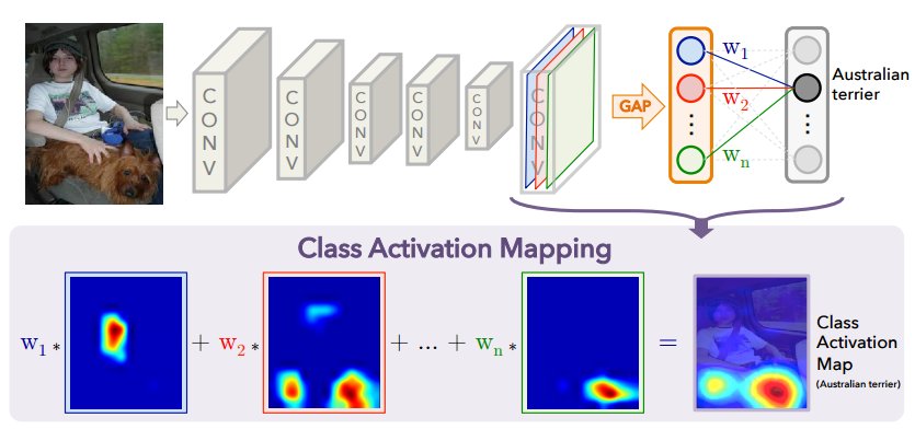
This result is the same as that of humans. Which part of the image does the human brain mainly focus on? For example, when we see a person, how do we judge that she is a woman? Of course, we look at the areas with obvious features such as the face, chest, and clothes. Based on this principle, it is called the “attention mechanism” in deep learning. There are many types of similar convolutional neural network visualizations, such as: Feature map visualization, weight visualization, Saliency map, etc. Here we will introduce weight visualization and feature map visualization.

The initial visualization work can be found in Imagenet classification…, which is the paper that proposed the AlexNet network used in the experiment. In this paper that开创了深度学习新纪元的论文, Krizhevshy directly visualized the convolutional kernels of the first convolutional layer. We can also reproduce this process. （注：“开创深度学习新纪元的论文”这里英文表述不太准确，可根据实际情况调整更合适的表达，比如“ushered in a new era of deep learning” ）

conv1_weights = list(model_saved.parameters())[0]
conv1_images = make_grid(conv1_weights, normalize=True).cpu()
plt.figure(figsize=(8, 8))
plt.imshow(conv1_images.permute(1, 2, 0).numpy())

<matplotlib.image.AxesImage at 0x7f4cb811da20>

The shape of the parameters of the convolutional kernels in the first layer of AlexNet implemented in PyTorch is a four-dimensional Tensor of \(64\times 3\times 11 \times 11\). In this way, we can obtain the above-mentioned 64 \(11\times 11\) image patches. Obviously, the information in these reconstructed images is basically about edges, stripes, and colors.

As we know, neural networks use convolutional kernels as feature extractors. Each convolutional kernel performs convolution on the input, generating a feature map. For example, the first convolutional layer of AlexNet has 64 convolutional kernels, so there are 64 feature maps.

The ideal feature map should be sparse and contain typical local information. Visualizing the feature map can provide some intuitive understanding and help debug the model. For example, if the feature map is very close to the original image, it means that it has not learned any features. If the feature map is almost a solid-color image, it means that it is too sparse, perhaps because the number of feature maps in the model is too large, which also reflects that the convolutional kernel is too small. We can adjust the parameters of the neural network based on this information.

Next, visualize the feature maps of the convolutional layers of AlexNet and write a general visualization function.

def visualize(alexnet, input_data, submodule_name, layer_index):
    """
    alexnet: 模型
    input_data: 输入数据
    submodule_name: 可视化 module 的 name, 专门针对 nn.Sequential
    layer_index: 在 submodule 中的 index
    """
    x = input_data
    modules = alexnet._modules
    for name in modules.keys():
        if name == submodule_name:
            module_layers = list(modules[name].children())
            for i in range(layer_index + 1):
                if type(module_layers[i]) == torch.nn.Linear:
                    x = x.reshape(x.size(0), -1)  # 针对线性层
                x = module_layers[i](x)
            return x

        x = modules[name](x)

Then, we can try to visualize the first convolutional layer.

feature_maps = visualize(model_saved, IMAGE.to(dev), "features", 0)
feature_images = make_grid(feature_maps.permute(1, 0, 2, 3), normalize=True).cpu()
plt.figure(figsize=(8, 8))
plt.imshow(feature_images.permute(1, 2, 0).numpy())

<matplotlib.image.AxesImage at 0x7f4cb8182d40>

62.10. Summary

There is a lot of content in this experiment. We have learned about the relevant knowledge of transfer learning, with a focus on introducing concepts such as fine-tuning, overfitting, underfitting, and their solutions. These concepts are basically used in actual development and applications. During actual training, we rarely start training from scratch. Instead, we often use pre-trained models that have already been trained. Therefore, we need to have a full grasp of this experiment.

Related Links

• Overfitting

• Classification: Instant Recognition with Caffe

• How to extract features of an image from a trained model

• Convolutional Neural Networks for Visual Recognition

---

○ Sharethis article link to your social media, blog, forum, etc. More external links will increase the search engine ranking of this site.

If you find this content helpful, you can buy me a coffee

Previous

61. Build the LeNet-5 Estimator

Next

63. Transfer Learning for Animal Classification