
88. Basic Linear Algebra in Python#
88.1. Introduction#
Linear algebra is a branch of mathematics that studies vector spaces and linear mappings. Linear algebra has wide applications in science and engineering because it can be used to solve many problems. In this tutorial, we will learn some basic knowledge of linear algebra, including vectors, matrices, determinants, eigenvalues, and eigenvectors, etc. At the same time, we will use Python code to implement these common linear algebra operations.
88.2. Key Points#
Vectors, Scalars, and Tensors
Matrix Operations
Python’s Broadcasting Mechanism
Identity Matrix
Matrix Transpose and Inverse
-
Eigenvalue Decomposition and Singular Value Decomposition
Principal Component Analysis
88.3. Vectors, Scalars, Matrices, and Tensors#
In mathematics, the variables we encounter are generally divided into the following categories:
-
Scalar: Simply put, a scalar is actually a single number. For example, if \(x = 5\), then \(x\) is a scalar, which has no physical meaning.
-
Vector: An ordered sequence of numbers arranged in a column or a row (a vector is composed of multiple scalars). For example, \(X=\left[\begin{array}{l}x_1\\x_2\\\vdots\\x_n\end{array}\right]\), where \(X\) is a vector.
-
Matrix: A two-dimensional array composed of multiple vectors. For example, \(X = \left[ \begin{array}{l}x_{11}&x_{12}&x_{13}\\x_{21}&x_{22}&x_{23}\end{array} \right]\), where \(X\) is a \(2\times3\) (number of rows × number of columns) matrix. Among them, the element in the \(i\)-th row and \(j\)-th column can be denoted as \(X_{i,j}\).
-
Tensor: A multi-dimensional array with three or more dimensions. For a tensor \(A\), the element with coordinates \((i, j, k)\) can be denoted as \(A_{i,j,k}\).
In summary, we can easily distinguish vectors (1D arrays), matrices (2D arrays), and tensors (multi-dimensional arrays) by the dimensions of the arrays.
We can also use the same function to initialize these variables (just by passing in different dimensions), and the code is as follows:
import numpy as np
# 向量
a = np.array([1, 2])
# 矩阵
b = np.array([[1, 2, 3], [4, 5, 6]])
#  在二维矩阵的基础上再加了一维, 形成张量
c = np.array([b, b])
print("向量 a 的大小:", a.shape)
print("矩阵 b 的大小:", b.shape)
print("张量 c 的大小:", c.shape)
向量 a 的大小: (2,)
矩阵 b 的大小: (2, 3)
张量 c 的大小: (2, 2, 3)
Among these variable types, the most frequently used one is the matrix. The pictures we take are matrices, the data we store in Excel are matrices, and the data we display from the database are also matrices. Moreover, every machine learning algorithm we have learned directly or indirectly involves matrices. Therefore, the study of matrices is of crucial importance.
88.4. Matrix Arithmetic Rules#
88.5. Operations between Matrices and Scalars#
Regardless of any operation of addition, subtraction, multiplication, or division, the operation between a scalar and a matrix can be expressed as: the scalar performs an operation on each element in the matrix. The code is as follows:
# 矩阵
a = np.array([[1, 2, 3], [4, 5, 6]])
print("a:\n", a)
print("a+2:\n", a+2)
print("a-2:\n", a-2)
print("a*2:\n", a*2)
print("a/2:\n", a/2)
a:
 [[1 2 3]
 [4 5 6]]
a+2:
 [[3 4 5]
 [6 7 8]]
a-2:
 [[-1  0  1]
 [ 2  3  4]]
a*2:
 [[ 2  4  6]
 [ 8 10 12]]
a/2:
 [[0.5 1.  1.5]
 [2.  2.5 3. ]]
88.6. Addition, Subtraction and Division between Matrices#
Condition: Only two matrices of equal size can be added or subtracted. That is, when one matrix is of size \(m\times n\), the other matrix must also be of size \(m\times n\).
Operation method: The elements in the corresponding positions of each matrix are operated on. Taking addition as an example, it is as follows:
Code test: Similar to adding and subtracting constants, you
can directly use the
+,
-,
/
operators:
# 矩阵
a = np.array([[1, 2, 3], [4, 5, 6]])
b = np.array([[1, 2, 3], [4, 5, 6]])
print("{}\n+\n{}\n=\n{}".format(a, b, a+b))
print("==============")
print("{}\n ÷ \n{}\n=\n{}".format(a, b, a/b))
[[1 2 3]
 [4 5 6]]
+
[[1 2 3]
 [4 5 6]]
=
[[ 2  4  6]
 [ 8 10 12]]
==============
[[1 2 3]
 [4 5 6]]
 ÷
[[1 2 3]
 [4 5 6]]
=
[[1. 1. 1.]
 [1. 1. 1.]]
88.7. Traditional Matrix Multiplication#
Condition: Matrix \(A\) can be multiplied by matrix \(B\) only when the size of \(A\) is \(m\times n\) and the size of \(B\) is \(n\times f\) (i.e., the number of columns of \(A\) is equal to the number of rows of \(B\)), and the size of the resulting product is necessarily \(m\times f\).
Operation method: Assume \(C = A\cdot B\), then the specific operation is defined as follows:
Simply put, the value of the \(i\)-th row and \(j\)-th column of matrix \(C\) is equal to the sum of the products of all the values in the \(i\)-th row of matrix \(A\) and all the values in the \(j\)-th column of matrix \(B\). For example:
From the above example, we can see that when the size of matrix \(A\) is \(2\times 3\) and the size of matrix \(B\) is \(3\times 2\), the size of the resulting product matrix \(C\) is \(2\times 2\). And the value of \(C_{12}\) is the sum of the products of the elements in the first row of matrix \(A\) and the second column of matrix \(B\), that is: \(1\times 4 + 2\times 5 + 3\times 6 = 32\). The calculation methods for other positions are similar.
Matrix multiplication satisfies the associative law and the distributive law, but does not satisfy the commutative law. As shown above, the size of the product matrix of \(AB\) is \(2\times 2\), but the size of \(BA\) becomes \(3\times 3\).
We can use the
dot
function to implement matrix multiplication:
a = np.array([[1, 2, 3], [4, 5, 6]])
b = np.array([[1, 4], [2, 5], [3, 6]])
# a 乘以 b
c = a.dot(b)
# b 乘以 a
d = b.dot(a)
print("ab的大小为:", c.shape)
print("值为:\n", c)
print("===========")
print("ba的大小为:", d.shape)
print("值为:\n", d)
ab的大小为: (2, 2)
值为:
 [[14 32]
 [32 77]]
===========
ba的大小为: (3, 3)
值为:
 [[17 22 27]
 [22 29 36]
 [27 36 45]]
88.8. Extended Operation: Hadamard Product#
According to the above knowledge, we know that the traditional matrix product is not the product of elements in the same positions of the matrices. However, sometimes we do need the product of corresponding elements. Therefore, mathematicians have proposed another product method called Hadamard to represent the product of corresponding elements, denoted as \(A\odot B\).
Of course, if we want to use this kind of product, it is necessary to ensure that the sizes of matrix \(A\) and matrix \(B\) are the same, so as to ensure that each element has a corresponding element to multiply.
We can use
np.multiply()
to implement it:
a = np.array([[1, 2, 3], [4, 5, 6]])
b = np.array([[1, 2, 1], [2, 2, 1]])
np.multiply(a, b)
array([[ 1,  4,  3],
       [ 8, 10,  6]])
As can be seen from the results, this method is the same as matrix addition, subtraction, and division. However, note that the matrix multiplication generally referred to in machine learning is the traditional matrix product. This product method is only used when the Hadamard matrix product is deliberately marked.
88.9. Extended Operation: Broadcasting Mechanism#
Through the above learning, we can know that a two-dimensional array and a one-dimensional array cannot be added because their positions cannot correspond one by one. However, NumPy provides us with a mechanism called the broadcasting mechanism that can achieve the addition of arrays with different sizes.
Of course, it is worth noting that this mechanism does not exist in mathematics and is only introduced for the convenience of programming.
Simply put, the broadcasting mechanism is to expand the shape of the smaller array to the shape of the larger array before performing operations on two arrays with different sizes, and then perform the operations. As shown below:
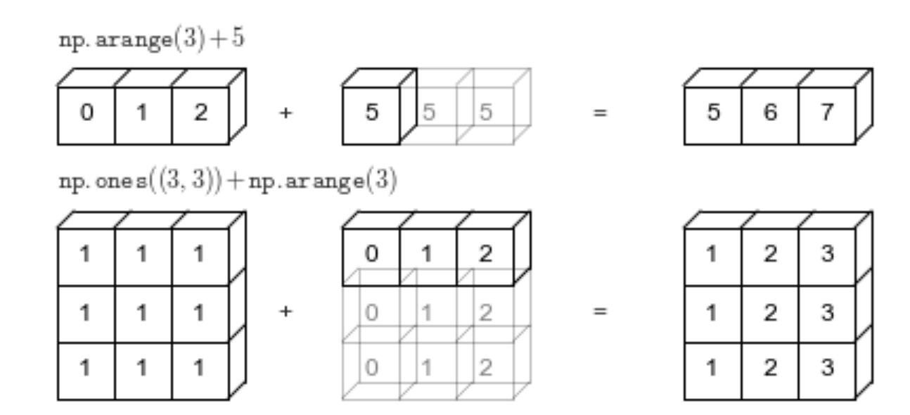
As shown above:
-
When a one-dimensional vector is operated on with a number, the number is replicated multiple times until it is equal in length to the vector before the calculation is performed.
-
When a two-dimensional array is operated on with a one-dimensional vector, if the length of the vector is equal to a certain dimension of the two-dimensional array, then the vector is assigned values until its size is the same as that of the two-dimensional array. Only then is the operation performed.
When we write code, NumPy automatically uses this mechanism:
a = np.array([[1, 2, 3], [4, 5, 6]])
b = np.array([[1, 2, 3]])
a+b
array([[2, 4, 6],
       [5, 7, 9]])
It is worth noting that not all matrix additions of
different sizes can be broadcast. If the dimensions of the
two arrays are different in any dimension and neither is
equal to 1, then broadcasting cannot be performed. NumPy
will return an error of
operands
                      could
                      not be
                      broadcast
                      together
                      with
                      shapes
.
# 两个数组的尺寸在任何维度都不相同,且都不等于 1
a_ = np.array([[1, 2, 3], [4, 5, 6]])
b_ = np.array([[1, 2]])
a_+b_
---------------------------------------------------------------------------
ValueError                                Traceback (most recent call last)
Cell In[7], line 4
      2 a_ = np.array([[1, 2, 3], [4, 5, 6]])
      3 b_ = np.array([[1, 2]])
----> 4 a_+b_

ValueError: operands could not be broadcast together with shapes (2,3) (1,2)
88.10. Properties of Matrices#
88.11. Transpose of a Matrix#
The new matrix obtained by interchanging the rows and columns of a matrix is called the transpose matrix, denoted as \(A^T\). An example is as follows:
As shown above, the transpose of a matrix is to turn the vector of the first row of the original matrix into a vector of one column, the vector of the second row of the original matrix into a vector of two columns, until all row vectors become column vectors.
Of course, it is very simple to implement it using NumPy. We
only need to add
.T
after the variable. As follows:
print("a:")
print(a)
print("a 的转置矩阵:")
print(a.T)
a:
[[1 2 3]
 [4 5 6]]
a 的转置矩阵:
[[1 4]
 [2 5]
 [3 6]]
88.12. Identity Matrix#
Identity Matrix: The \(n\)-order identity matrix is an \(n\times n\) square matrix (i.e., a matrix with the same number of rows and columns), where the elements on the main diagonal are 1 and the rest are 0. The identity matrix is generally denoted as \(I_n\). The form is as follows:
You can directly use
np.identity()
to define an identity matrix:
# 传入大小 n
np.identity(4)
array([[1., 0., 0., 0.],
       [0., 1., 0., 0.],
       [0., 0., 1., 0.],
       [0., 0., 0., 1.]])
88.13. Inverse of a Matrix#
The inverse matrix of the square matrix \(A\) is denoted as \(A^{-1}\), and this matrix satisfies the following conditions:
That is to say, if the product (conventional product) of a matrix and \(A\) is an identity matrix, then this matrix is the inverse matrix of \(A\).
Regarding the specific method of finding the inverse matrix of \(A\) in mathematics specific method, it will not be elaborated here. We directly use NumPy to find it:
a = np.array([[1, 2], [3, 4]])
# 通过 np.linalg.inv() 求取逆矩阵
print(np.linalg.inv(a))
print("=================")
# 矩阵对象可以通过 ‘.I’ 属性,更方便的求逆
A = np.matrix(a)
print(A.I)
[[-2.   1. ]
 [ 1.5 -0.5]]
=================
[[-2.   1. ]
 [ 1.5 -0.5]]
As above, we provided two ways to find the inverse matrix.
Generally, we call the above-mentioned invertible matrix a non-singular matrix and the non-invertible matrices singular matrices. There are many ways to distinguish whether a matrix is invertible, and the most commonly used one is to judge the determinant of the matrix.
-
If the matrix is a square matrix and the determinant of the square matrix is not equal to 0, it means the matrix is invertible.
-
Otherwise, it is non-invertible (i.e., a singular matrix).
88.14. Determinant of a Matrix#
The determinant is a characteristic only possessed by square matrices (i.e., matrices with an equal number of rows and columns), denoted as \(det(A)\) or also as \(|A|\). Its calculation formula is relatively complex and is a nightmare for many students in school. Of course, as a programmer, we don’t need to be familiar with the specific calculation steps of this determinant. We only need to know how to find and use it.
We can use
np.linalg.det()
to calculate the determinant:
a = np.array([[1, 2], [3, 4]])
b = np.array([[1, 2], [2, 4]])
print("a的行列式为", np.linalg.det(a))
print("b的行列式为", np.linalg.det(b))
a的行列式为 -2.0000000000000004
b的行列式为 0.0
From the above results, it can be seen that the determinant
of matrix a is not 0, so it is an invertible matrix. While
the determinant of matrix b is 0, so it is a non-invertible
matrix. You can try to use the
np.linalg.inv()
method to find the inverse matrix of b and observe whether
the program reports an error.
88.15. Norm#
In machine learning, we often need to use norms to measure the magnitude of vectors. There are many forms of norms, and the L2 norm, also known as the Euclidean norm, is often used in machine learning. The calculation formula for this norm is as follows:
According to the formula, it is not difficult for us to find that the L2 norm of a vector is actually the square root of the sum of the squares of the absolute values.
In addition to being applied to traditional machine learning, such as ridge regression and Bayesian inference, the L2 norm is also widely used in deep learning. For example, regularization using the L2 norm can effectively alleviate the decay of neural network weights and improve the generalization ability of the model.
We can calculate the L2 norm using
np.linalg.norm():
print("按列向量计算 a 的范数", np.linalg.norm(a, axis=0))  # 按列向量计算范数
print("按行向量计算 a 的范数", np.linalg.norm(a, axis=1))  # 按行向量计算范数
print("计算矩阵 a 的范数", np.linalg.norm(a))  # 按列向量计算范数
按列向量计算 a 的范数 [3.16227766 4.47213595]
按行向量计算 a 的范数 [2.23606798 5.        ]
计算矩阵 a 的范数 5.477225575051661
88.16. Trace of a Matrix#
The trace of a matrix is the sum of the diagonal elements (i.e., all the elements on the diagonal) of the matrix, denoted as \(Tr(A)\). The calculation formula is as follows:
We can use
np.trace()
to quickly obtain the trace of a matrix as follows:
print("a_00:", a[0][0])
print("a_11:", a[1][1])
print("Tr(a):", np.trace(a))
a_00: 1
a_11: 4
Tr(a): 5
88.17. Special Matrices#
Diagonal Matrix: A matrix that has non-zero elements only on the main diagonal and zeros everywhere else. In fact, it is very similar to the identity matrix above, except that the elements on the diagonal of the identity matrix must be 1, while the elements on the diagonal of a diagonal matrix can be any non-zero value. Therefore, the form of a diagonal matrix \(diag(x)\) is as follows:
We can directly use
np.diag()
to define a diagonal matrix:
# 函数传入的是对角线上的值
x = np.diag((1, 2, 3, 4))
x
array([[1, 0, 0, 0],
       [0, 2, 0, 0],
       [0, 0, 3, 0],
       [0, 0, 0, 4]])
Interestingly, in addition to creating a diagonal matrix, this function can also extract the values on the diagonal from a diagonal matrix:
np.diag(x)
array([1, 2, 3, 4])
Symmetric Matrix: If the transpose of matrix \(A\) is the same as matrix \(A\), then matrix \(A\) is a symmetric matrix. In other words, if matrix \(A\) satisfies \(A_{ij} = A_{ji}\), where \(i\) and \(j\) are arbitrary values, then \(A\) is a symmetric matrix.
Because the transposes are the same, the number of rows of matrix \(A\) must be equal to the number of columns, that is, the matrix must be a square matrix. Because of symmetry, the contents of the upper triangle (the triangular content above the diagonal) and the lower triangle must be symmetric. As shown below:
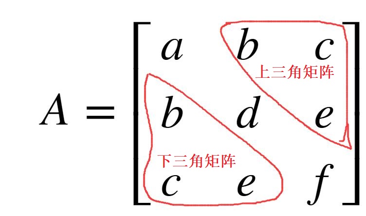
As can be seen from the above example, this matrix is symmetric along the diagonal, and the content of the upper triangle of the matrix is equal to the content of the lower triangle of the matrix.
However, there is no ready-made library in NumPy to directly create a symmetric matrix. The steps to create a symmetric matrix are as follows:
First, let’s initialize a \(5 \times 5\) matrix:
# 随机初始化 25 个数,然后将这一组数转换为 5*5 的矩阵
x = np.random.randn(25).reshape(5, 5)
x
array([[-1.76147734, -0.86482382,  0.62757387, -1.30881442, -2.1407301 ],
       [-1.95812775, -0.02321958,  0.6240782 , -0.48150296,  0.90741739],
       [-0.03717522, -1.26331227,  1.10608778,  0.39242673, -1.16064422],
       [ 1.1341177 , -1.81348565,  0.92502167,  1.95435312, -0.05584964],
       [-1.54326738,  1.16051111,  1.1648892 , -2.28413737,  0.50776626]])
Then use the
triu()
function to extract the upper triangular matrix of matrix x:
cov_up = np.triu(x)
cov_up
array([[-1.76147734, -0.86482382,  0.62757387, -1.30881442, -2.1407301 ],
       [ 0.        , -0.02321958,  0.6240782 , -0.48150296,  0.90741739],
       [ 0.        ,  0.        ,  1.10608778,  0.39242673, -1.16064422],
       [ 0.        ,  0.        ,  0.        ,  1.95435312, -0.05584964],
       [ 0.        ,  0.        ,  0.        ,  0.        ,  0.50776626]])
Next, we need to transpose the upper triangular matrix to obtain the symmetric lower triangular matrix, as follows:
cov_down = cov_up.T
cov_down
array([[-1.76147734,  0.        ,  0.        ,  0.        ,  0.        ],
       [-0.86482382, -0.02321958,  0.        ,  0.        ,  0.        ],
       [ 0.62757387,  0.6240782 ,  1.10608778,  0.        ,  0.        ],
       [-1.30881442, -0.48150296,  0.39242673,  1.95435312,  0.        ],
       [-2.1407301 ,  0.90741739, -1.16064422, -0.05584964,  0.50776626]])
Then, we can add the upper triangular matrix and the lower triangular matrix together:
cov_up_down = cov_up+cov_down
cov_up_down
array([[-3.52295468, -0.86482382,  0.62757387, -1.30881442, -2.1407301 ],
       [-0.86482382, -0.04643916,  0.6240782 , -0.48150296,  0.90741739],
       [ 0.62757387,  0.6240782 ,  2.21217556,  0.39242673, -1.16064422],
       [-1.30881442, -0.48150296,  0.39242673,  3.90870625, -0.05584964],
       [-2.1407301 ,  0.90741739, -1.16064422, -0.05584964,  1.01553252]])
Careful you may have noticed that although this can get a
symmetric matrix, we added the diagonal values twice (the
diagonal values in both the upper triangular matrix and the
lower triangular matrix exist). Therefore, finally, we need
to subtract a diagonal value from the obtained
cov_up_down.
First, let’s initialize a diagonal matrix with only diagonal elements having values:
# 获得对角线的值
d = np.diag(x)
# 获得对角矩阵
dia = np.diag(d)
dia
array([[-1.76147734,  0.        ,  0.        ,  0.        ,  0.        ],
       [ 0.        , -0.02321958,  0.        ,  0.        ,  0.        ],
       [ 0.        ,  0.        ,  1.10608778,  0.        ,  0.        ],
       [ 0.        ,  0.        ,  0.        ,  1.95435312,  0.        ],
       [ 0.        ,  0.        ,  0.        ,  0.        ,  0.50776626]])
Finally, subtract a diagonal matrix to obtain the final symmetric matrix:
x = cov_up_down-dia
x
array([[-1.76147734, -0.86482382,  0.62757387, -1.30881442, -2.1407301 ],
       [-0.86482382, -0.02321958,  0.6240782 , -0.48150296,  0.90741739],
       [ 0.62757387,  0.6240782 ,  1.10608778,  0.39242673, -1.16064422],
       [-1.30881442, -0.48150296,  0.39242673,  1.95435312, -0.05584964],
       [-2.1407301 ,  0.90741739, -1.16064422, -0.05584964,  0.50776626]])
We can use the fact that the transpose of a matrix is equal to the matrix itself to test whether x is a symmetric matrix:
x == x.T
array([[ True,  True,  True,  True,  True],
       [ True,  True,  True,  True,  True],
       [ True,  True,  True,  True,  True],
       [ True,  True,  True,  True,  True],
       [ True,  True,  True,  True,  True]])
Orthogonal Matrix: When a square matrix \(A\) satisfies \(A^TA = AA^T=I\), \(A\) is called an orthogonal matrix.
According to the definition of the inverse matrix, if a matrix is invertible, then \(A^{-1}A = I\). Therefore, combining the above two equations, if matrix \(A\) is both an inverse matrix and an orthogonal matrix, then we have:
88.18. Matrix Decomposition#
88.19. Eigenvalues and Eigen Decomposition#
Do you still remember the composition of forces we learned in high school? Force \(\vec{j}\) and force \(\vec{i}\) can be superimposed to obtain force \(\vec{A}\), denoted as \((\vec{i}, \vec{j})\), as shown in Figure 1 below:
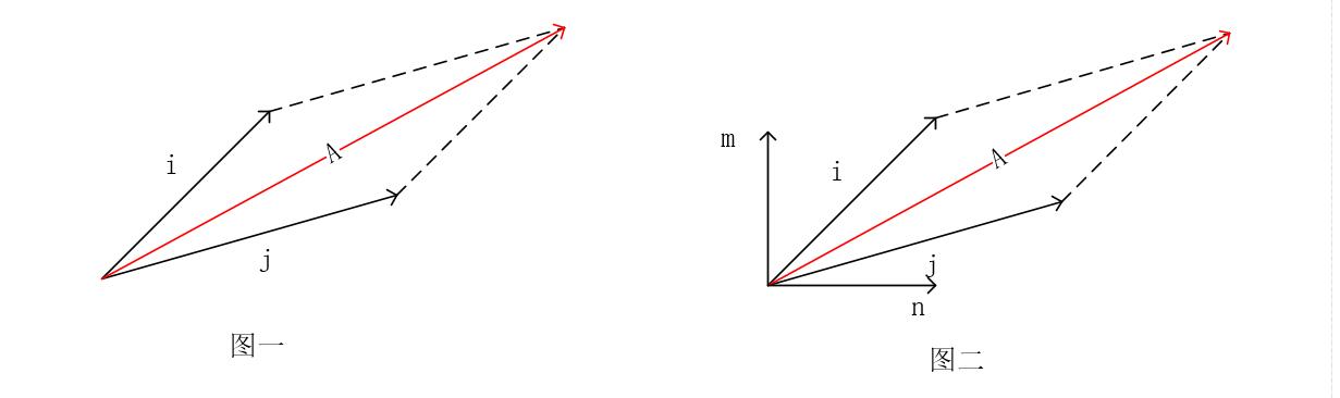
As can be seen from Figure 1, when taking \(i\) and \(j\) as the coordinate axes, \(\vec{A}\) can be expressed as \(1\vec{i} + 1\vec{j}\). In other words, in the coordinate space of \(i\) and \(j\), the coordinates of \(\vec{A}\) are \((1i, 1j)\).
However, obviously, the resultant force \(\vec{A}\) expressed using \(i\) and \(j\) cannot well demonstrate the effect of the force on the object (i.e., how much the object will move upward and how much it will move to the right under this force). Therefore, we often make another transformation, decomposing the force into two directions: horizontal and vertical, that is, transforming the force \(\vec{A}\) into the coordinate space of \(\vec{m}\) and \(\vec{n}\) shown in Figure 2. Then, at this time, the coordinates of \(\vec{A}\) are no longer \((1i, 1j)\), but \((\lambda_1m, \lambda_2n)\).
The principle of eigen decomposition is similar to that of force decomposition, which is the process of transforming a square matrix \(A\) into a matrix in a new space. The coordinate axis vectors in the new space are called eigenvectors (denoted as \(v\)), and the multiples of the matrix \(A\) and the eigenvectors are called eigenvalues, denoted as \(\lambda\) (i.e., the set of \(\lambda_1, \lambda_2,...\) above).
We can use \(\lambda v\) to represent the coordinates of the square matrix \(A\) in the new space. Similarly, according to the physical properties of matrix multiplication, we can also use \(A\cdot v\) to represent the process of transforming the original square matrix \(A\) into the new space with the eigenvector \(v\).
Therefore, the matrix \(A\) and its eigenvectors and eigenvalues must satisfy the following equation:
Suppose the set of eigenvectors of the square matrix \(A\) is \(V = \{v_1, v_2,..., v_n\}\), and the set of eigenvalues is \(\lambda = \{\lambda_1, \lambda_2,..., \lambda_n\}\). According to the above equation, we can obtain the following relationship for \(A\) (multiplying both sides of the equation by \(V^{-1}\) on the right):
Given \(A\), the algorithm for solving \(V\) and \(\lambda\) above is very complex and requires the use of relevant knowledge such as the orthogonal matrix and diagonal matrix above. You can refer to this article.
Here, we directly use the
vals,
                      vecs =
                      np.linalg.eig(x)
function to complete the eigenvalue decomposition and solve
for the specific values of
\(V\) and
\(\lambda\). This function has two main return values:
-
The first returned variable is the eigenvalues obtained from the decomposition.
-
The second returned variable is the eigenvectors corresponding to each eigenvalue.
a = np.array([[1, 2, 3], [5, 8, 7], [1, 1, 1]])
e_vals, e_vecs = np.linalg.eig(a)
print("特征值为:", e_vals)
print("特征向量为:\n", e_vecs)
特征值为: [10.254515   -0.76464793  0.51013292]
特征向量为:
 [[-0.24970571 -0.89654947  0.54032982]
 [-0.95946634  0.19306928 -0.73818337]
 [-0.13065753  0.39865186  0.40389232]]
As shown above, the matrix \(a\) is decomposed into the eigenvalues \(e\_vals\) and the eigenvectors \(e\_vecs\), with one eigenvector corresponding to one eigenvalue.
So what exactly are the uses of the obtained eigenvalues and eigenvectors in machine learning?
From the above learning, we can easily obtain the following conclusion: Eigenvalue decomposition actually separates the vector directions and distances in the original matrix. We can obtain the eigenvalues on each eigenvector, and then compare the contribution degrees of each group of vectors (eigenvector + eigenvalue) to the content of the original matrix.
Taking the above test code as an example, we have obtained the three eigenvalues of matrix \(a\) and their corresponding eigenvectors. Now let’s calculate the percentage of each eigenvalue in the total eigenvalues and then estimate the contribution degree of each eigenvector to the original matrix (here, the eigenvalues need to be made absolute first and then summed. Because the positive and negative signs here only represent directions).
pro = abs(e_vals)/np.sum(abs(e_vals))
pro
array([0.88943116, 0.06632217, 0.04424667])
As can be seen from the above, the contribution degree of the first group (eigenvector + eigenvalue) to the content of the original matrix can reach 89%, while the other two groups are only 6.6% and 4.4%. Of course, since the matrix here is just a \(3\times 3\) matrix, it is difficult for us to see the great role of eigenvalue decomposition.
But imagine if this matrix is a \(1000\times1000\) matrix. When it is eigenvalue decomposed into eigenvalues + eigenvectors, the sum of the contribution degrees of two groups of eigenvalues + eigenvectors to the content of the original matrix is 89%, while the sum of the contributions of the other 998 groups is only 11%. Then, can we delete those eigenvalues + eigenvectors with relatively small contribution degrees to the content of the original matrix?
That is to say, we can use two groups of eigenvalues + eigenvectors to represent 89% of the content of this \(1000\times1000\) matrix. This is data dimensionality reduction, which is the process of reducing the amount of data and the number of data features while preserving most of the original data content.
Of course, it doesn’t mean that all matrices can be eigenvalue decomposed. Eigenvalue decomposition is only effective when the matrix is an invertible square matrix.
However, the data we encounter in daily life is rarely a complete square matrix. It may have only 100 features, but 10,000 data entries for each feature. Therefore, next we will introduce a more general matrix decomposition method: Singular Value Decomposition (SVD).
88.20. Singular Value Decomposition#
Singular Value Decomposition (SVD) is also a matrix decomposition method, which can decompose a matrix into singular vectors and singular values. Singular value decomposition is not only a mathematical problem but also widely applied in the engineering field. For example, in some current recommendation systems.
The singular value decomposition process of any real matrix \(A\) can be expressed as:
Among them, \(D\) is a diagonal matrix, and the elements on its diagonal are called singular values. The column vectors of matrix \(U\) are called “left singular vectors”, and the column vectors of matrix \(V\) are called “right singular vectors”. When we need to compress the number of rows of a matrix, the combination we use is: left singular vectors + singular values. When we perform dimensionality reduction by compressing the number of columns of a matrix, what we use is: right singular vectors + singular values.
Similarly, given \(A\), the mathematical derivation formulas for obtaining \(U\), \(D\), and \(V\) are very complex. Here, we directly use NumPy to solve it.
We use the
np.linalg.svd(a)
function to perform singular value decomposition on matrix
\(A\),
obtaining the following three return values:
-
The first return value: The left singular vectors \(U\) of matrix \(A\).
-
The second return value: The values on the diagonal of the diagonal matrix \(D\) (for a diagonal matrix, all values are 0 except those on the diagonal).
-
The third return value: The transpose \(V^T\) of the right singular vectors \(V\) of matrix \(A\).
a = np.array([[1, 2, 3, 4], [5, 8, 6, 7], [1, 1, 1, 2]])
u, s, vh = np.linalg.svd(a)  # vh 表示 v 的转置
print(u.shape, s.shape, vh.shape)
(3, 3) (3,) (4, 4)
Now we can verify whether the singular values and singular vectors obtained using NumPy truly satisfy the singular decomposition formula and can fully represent the content of the original matrix.
First, let’s convert \(s\) into a diagonal matrix \(D\). To be able to multiply \(U\) on the left and \(V^T\) on the right, the size of the generated diagonal matrix \(D\) must be \(3\times4\).
# 初始化 3×4 全为 0 的矩阵
D = np.zeros((3, 4))
# np.diag(s) 只能生成 3×3 的矩阵
D[:3, :3] = np.diag(s)
D
array([[14.37981705,  0.        ,  0.        ,  0.        ],
       [ 0.        ,  1.97748535,  0.        ,  0.        ],
       [ 0.        ,  0.        ,  0.55714755,  0.        ]])
Finally, multiply them and observe whether the resulting value is the same as \(A\).
# 但传入的两个变量之间的差距在 0.00001 以内时,返回true
np.allclose(a, np.dot(u, np.dot(D, vh)))
True
So far, I have finished learning the linear algebra knowledge used in machine learning. Next, let’s use the learned linear algebra knowledge to implement the PCA algorithm and complete the visualization of the Iris dataset.
88.21. Visualization of the Iris Dataset#
88.22. Introduction to the Dataset#
The Iris dataset is one of the most commonly used datasets in machine learning. This dataset contains three classes of Iris flowers, with a total of 150 data entries. Each data entry records four features of a flower, namely the sepal length, sepal width, petal length, and petal width, and also indicates which type of Iris flower it belongs to.
Let’s use the scikit-learn library to load this dataset:
from sklearn import datasets
iris = datasets.load_iris()
# 加载特征
iris_data = iris['data']
# 加载标签
iris_label = iris['target']
print(iris_data.shape)
print(iris_label.shape)
(150, 4)
(150,)
Among them, the
iris_data
variable stores the four features of 150 flowers, and
iris_label
represents the types of these 150 flowers respectively.
Next, we want to plot these sample points in a coordinate system to observe the relationship between the data points and the types of flowers. However, since the flower has four features and we can at most draw graphs in three-dimensional space. Therefore, we need to reduce the dimension of the original dataset so that its dimension is reduced to 2 or 3, so that we can perform visualization. And here, the dimensionality reduction method we use is the Principal Component Analysis (PCA).
88.23. Principal Component Analysis#
Principal Component Analysis (PCA) is a machine learning algorithm for data compression. This algorithm can decompose high-dimensional variables with linear correlation into low-dimensional variables that are linearly independent. The new low-dimensional variables can retain most of the information of the original data, thus achieving the effect of dimensionality reduction.
There are two main implementation methods of the Principal Component Analysis method. One is based on eigenvalue decomposition, and the other is based on singular value decomposition.
The specific steps of based on singular value decomposition are as follows:
-
Center the sample data to obtain the data \(x\).
-
Perform SVD (Singular Value Decomposition) on \(x\) to obtain \(u\), \(s\), and \(v\).
-
Take the first \(d\) right singular vectors of \(v\), denoted as \(v[0:d]\).
-
\(x\cdot v[0:d]\) is the data in the low-dimensional space (it can also be obtained by multiplying the singular values by the singular vectors).
The centering process here is to subtract the mean of its own dimension from each element value. This can make the mean of each dimension of the input data be 0 (due to the existence of decimals, it may be infinitely close to 0 but not equal to 0), thereby increasing the robustness of the data. As follows:
data_cen = iris_data - np.mean(iris_data, axis=0)  # 样本中心化处理
# 去中心化后的矩阵的每个维度的平均值无限接近于 0
np.mean(data_cen, axis=0)
array([-1.12502600e-15, -7.60872846e-16, -2.55203266e-15, -4.48530102e-16])
Next, let’s complete the PCA function based on SVD according to the above steps:
def pca_svd(data):
    # 进行svd 分解
    u, s, v = np.linalg.svd(data)
    # 这里选取前两个特征v[0:2]
    # 然后计算低维空间数据
    pc_svd = np.dot(data, v[:, 0:2])
    return pc_svd


pc_svd = pca_svd(data_cen)
pc_svd
array([[-2.24698392,  1.46899397],
       [-1.99096685,  1.85097919],
       [-2.25276491,  1.78164249],
       [-2.10683872,  1.74352871],
       [-2.34878146,  1.40443007],
       [-2.16349706,  0.90825477],
       [-2.33046962,  1.55229906],
       [-2.15926072,  1.49067128],
       [-2.10600127,  1.96625659],
       [-2.02997146,  1.75014427],
       [-2.21168271,  1.23781384],
       [-2.17333505,  1.4477847 ],
       [-2.05865423,  1.89140375],
       [-2.41395648,  2.11303825],
       [-2.43871366,  1.16432965],
       [-2.49978144,  0.63739946],
       [-2.396309  ,  1.1474191 ],
       [-2.2154352 ,  1.43702166],
       [-2.02097092,  0.98788647],
       [-2.35420885,  1.15818214],
       [-1.89830011,  1.33728011],
       [-2.25700125,  1.19922598],
       [-2.72614803,  1.67740341],
       [-1.84641105,  1.33973607],
       [-1.99872609,  1.26841145],
       [-1.83842222,  1.72294477],
       [-2.03796029,  1.36693557],
       [-2.15264228,  1.40075063],
       [-2.14518638,  1.53355786],
       [-2.07815596,  1.60226924],
       [-1.97635842,  1.66683313],
       [-1.95160864,  1.39291765],
       [-2.57814426,  0.99462608],
       [-2.56204142,  0.92407196],
       [-1.99842274,  1.71817196],
       [-2.20255192,  1.81607681],
       [-2.16063227,  1.49497604],
       [-2.41646883,  1.44485464],
       [-2.22986313,  1.95303153],
       [-2.12312206,  1.48221903],
       [-2.30977685,  1.50526499],
       [-1.70256362,  2.42371997],
       [-2.36118089,  1.80699924],
       [-2.04052173,  1.22997481],
       [-2.08984819,  0.8870455 ],
       [-1.99555679,  1.82745913],
       [-2.32755458,  1.13036337],
       [-2.23070058,  1.73030365],
       [-2.24782137,  1.24626609],
       [-2.15180483,  1.6234785 ],
       [ 0.93591038, -0.82932384],
       [ 0.63422117, -0.69100048],
       [ 1.11338528, -0.89940993],
       [ 0.54579077,  0.40511511],
       [ 0.99119832, -0.46717924],
       [ 0.58078863, -0.27582553],
       [ 0.68037832, -0.90711885],
       [-0.23876712,  0.89726699],
       [ 0.89858067, -0.48470301],
       [ 0.14808502,  0.16622606],
       [ 0.17641302,  1.06129714],
       [ 0.41023667, -0.32333369],
       [ 0.69749678,  0.53178693],
       [ 0.80763908, -0.53420515],
       [-0.04483578,  0.19773033],
       [ 0.71854432, -0.5515777 ],
       [ 0.47642965, -0.47735018],
       [ 0.35512806,  0.12381963],
       [ 1.21853262,  0.05606546],
       [ 0.32931125,  0.37436628],
       [ 0.72278299, -0.9240294 ],
       [ 0.43432834, -0.01067912],
       [ 1.29050659, -0.41059956],
       [ 0.81020051, -0.39724439],
       [ 0.65169439, -0.28842526],
       [ 0.74806454, -0.4701093 ],
       [ 1.18447155, -0.58014585],
       [ 1.22806727, -0.93322498],
       [ 0.68664317, -0.43814304],
       [ 0.03543037,  0.56403452],
       [ 0.30062848,  0.51562575],
       [ 0.21087678,  0.60738915],
       [ 0.30181953,  0.17945718],
       [ 1.19872755, -0.68282957],
       [ 0.40415233, -0.46044568],
       [ 0.3898975 , -0.83519607],
       [ 0.924702  , -0.76292326],
       [ 1.06771198,  0.09833277],
       [ 0.18052027, -0.17424123],
       [ 0.41447301,  0.25908282],
       [ 0.55007736, -0.02112534],
       [ 0.68377721, -0.54743021],
       [ 0.42568139,  0.19268224],
       [-0.13696958,  0.96183088],
       [ 0.43569989, -0.01498388],
       [ 0.2433132 , -0.21051225],
       [ 0.34052079, -0.16946842],
       [ 0.57941707, -0.27152076],
       [-0.37520891,  0.95474728],
       [ 0.34797669, -0.03666119],
       [ 1.7209556 , -1.97215372],
       [ 1.22109639, -0.76184199],
       [ 2.02264365, -1.63304298],
       [ 1.52993814, -1.21711864],
       [ 1.77915743, -1.5545107 ],
       [ 2.61075784, -2.09384182],
       [ 0.61485086, -0.11704833],
       [ 2.29874562, -1.72017874],
       [ 2.05353425, -1.07844524],
       [ 1.90742989, -2.3270635 ],
       [ 1.17732134, -1.21806078],
       [ 1.55433431, -0.93213767],
       [ 1.68141573, -1.36852189],
       [ 1.28962122, -0.57953868],
       [ 1.31318111, -0.99471969],
       [ 1.35223481, -1.42510763],
       [ 1.47835359, -1.24724821],
       [ 2.21137718, -2.77818661],
       [ 3.1472384 , -2.05354736],
       [ 1.43727023, -0.22598545],
       [ 1.76574004, -1.70653322],
       [ 0.99830294, -0.73034378],
       [ 2.80486852, -1.98408055],
       [ 1.253835  , -0.65254877],
       [ 1.56470641, -1.69870024],
       [ 1.89102138, -1.75140167],
       [ 1.09383447, -0.65732158],
       [ 0.98458105, -0.8546927 ],
       [ 1.72638183, -1.24847168],
       [ 1.84283572, -1.42184259],
       [ 2.31568591, -1.56800499],
       [ 2.04594811, -2.55177324],
       [ 1.75793055, -1.28044399],
       [ 1.20993593, -0.74923015],
       [ 1.52844257, -0.85327647],
       [ 2.41897901, -1.86728327],
       [ 1.39093607, -1.77403322],
       [ 1.37655606, -1.3118121 ],
       [ 0.8902394 , -0.78644937],
       [ 1.59369253, -1.3901992 ],
       [ 1.73246734, -1.5887938 ],
       [ 1.48218101, -1.27477057],
       [ 1.22109639, -0.76184199],
       [ 1.84600735, -1.81766313],
       [ 1.69090129, -1.82658948],
       [ 1.53376555, -1.24464101],
       [ 1.47490445, -0.59827988],
       [ 1.36684208, -1.13181958],
       [ 1.20684272, -1.61402649],
       [ 1.0287097 , -0.95737037]])
As shown above, we have reduced the dimension of the original data and obtained two new columns of data. These two new columns of data can represent most of the content of the original data. Now, we can use a two-dimensional image to show the distribution of these 150 data points.
import matplotlib.pyplot as plt
%matplotlib inline
plt.scatter(pc_svd[:, 0], pc_svd[:, 1], c=iris_label)
plt.show()

The above figure intuitively shows the distribution of these three types of iris flowers. Of course, it is worth noting that these two new columns of data are different from any of the original columns of data. These two columns of data are two new columns of data generated from the information of the original four columns of data through SVD.
The steps of eigenvalue decomposition are similar to those of SVD-based decomposition. However, since only square matrices can be eigen-decomposed, we need to process the matrix once before performing eigen-decomposition to obtain its covariance matrix (the covariance matrix of any matrix is necessarily a square matrix). The specific steps are as follows:
-
Center the original dataset to obtain dataset X.
-
Calculate the covariance matrix \(XX^T\) of dataset X.
-
Perform eigen-decomposition on the covariance matrix \(XX^T\).
-
Select the eigenvectors corresponding to the largest \(d\) eigenvalues.
-
Multiply matrix X by these \(d\) eigenvectors to obtain the data in the low-dimensional space (alternatively, the data in the low-dimensional space can also be obtained by multiplying the selected eigenvalues by the eigenvectors).
Here we introduce a new concept, the covariance matrix. The formula for this matrix is \(XX^T\). Suppose the size of the original data X is \(m\times n\), then the size of \(X^T\) is \(n\times m\). Thus, the size of the covariance matrix \(XX^T\) is \(m\times m\), that is, \(XX^T\) is a square matrix. In this way, we can perform eigen-decomposition. Of course, we will cover more knowledge points about the covariance matrix in later statistics courses.
Based on the above description, let’s define the PCA function based on eigenvalue decomposition as follows:
def pca_eig(data_cen):
    # 计算协方差矩阵,每行为一个样本
    cov_mat = np.cov(data_cen, rowvar=0)
    eigVals, eigVects = np.linalg.eig(cov_mat)
    # 对特征值进行排序
    eigValInd = np.argsort(eigVals)
    # 排序是从小到大排序,因此选择最后面两个
    eigValInd = eigValInd[:-3:-1]
    # 得到投影矩阵,即对原内容来说,最为关键特征向量
    redEigVects = eigVects[:, eigValInd]
    # 通过投影矩阵得到降维后的数据
    pc_eig = np.dot(data_cen, redEigVects)
    return pc_eig


pc_eig = pca_eig(data_cen)
pc_eig
array([[-2.68412563, -0.31939725],
       [-2.71414169,  0.17700123],
       [-2.88899057,  0.14494943],
       [-2.74534286,  0.31829898],
       [-2.72871654, -0.32675451],
       [-2.28085963, -0.74133045],
       [-2.82053775,  0.08946138],
       [-2.62614497, -0.16338496],
       [-2.88638273,  0.57831175],
       [-2.6727558 ,  0.11377425],
       [-2.50694709, -0.6450689 ],
       [-2.61275523, -0.01472994],
       [-2.78610927,  0.235112  ],
       [-3.22380374,  0.51139459],
       [-2.64475039, -1.17876464],
       [-2.38603903, -1.33806233],
       [-2.62352788, -0.81067951],
       [-2.64829671, -0.31184914],
       [-2.19982032, -0.87283904],
       [-2.5879864 , -0.51356031],
       [-2.31025622, -0.39134594],
       [-2.54370523, -0.43299606],
       [-3.21593942, -0.13346807],
       [-2.30273318, -0.09870885],
       [-2.35575405,  0.03728186],
       [-2.50666891,  0.14601688],
       [-2.46882007, -0.13095149],
       [-2.56231991, -0.36771886],
       [-2.63953472, -0.31203998],
       [-2.63198939,  0.19696122],
       [-2.58739848,  0.20431849],
       [-2.4099325 , -0.41092426],
       [-2.64886233, -0.81336382],
       [-2.59873675, -1.09314576],
       [-2.63692688,  0.12132235],
       [-2.86624165, -0.06936447],
       [-2.62523805, -0.59937002],
       [-2.80068412, -0.26864374],
       [-2.98050204,  0.48795834],
       [-2.59000631, -0.22904384],
       [-2.77010243, -0.26352753],
       [-2.84936871,  0.94096057],
       [-2.99740655,  0.34192606],
       [-2.40561449, -0.18887143],
       [-2.20948924, -0.43666314],
       [-2.71445143,  0.2502082 ],
       [-2.53814826, -0.50377114],
       [-2.83946217,  0.22794557],
       [-2.54308575, -0.57941002],
       [-2.70335978, -0.10770608],
       [ 1.28482569, -0.68516047],
       [ 0.93248853, -0.31833364],
       [ 1.46430232, -0.50426282],
       [ 0.18331772,  0.82795901],
       [ 1.08810326, -0.07459068],
       [ 0.64166908,  0.41824687],
       [ 1.09506066, -0.28346827],
       [-0.74912267,  1.00489096],
       [ 1.04413183, -0.2283619 ],
       [-0.0087454 ,  0.72308191],
       [-0.50784088,  1.26597119],
       [ 0.51169856,  0.10398124],
       [ 0.26497651,  0.55003646],
       [ 0.98493451,  0.12481785],
       [-0.17392537,  0.25485421],
       [ 0.92786078, -0.46717949],
       [ 0.66028376,  0.35296967],
       [ 0.23610499,  0.33361077],
       [ 0.94473373,  0.54314555],
       [ 0.04522698,  0.58383438],
       [ 1.11628318,  0.08461685],
       [ 0.35788842,  0.06892503],
       [ 1.29818388,  0.32778731],
       [ 0.92172892,  0.18273779],
       [ 0.71485333, -0.14905594],
       [ 0.90017437, -0.32850447],
       [ 1.33202444, -0.24444088],
       [ 1.55780216, -0.26749545],
       [ 0.81329065,  0.1633503 ],
       [-0.30558378,  0.36826219],
       [-0.06812649,  0.70517213],
       [-0.18962247,  0.68028676],
       [ 0.13642871,  0.31403244],
       [ 1.38002644,  0.42095429],
       [ 0.58800644,  0.48428742],
       [ 0.80685831, -0.19418231],
       [ 1.22069088, -0.40761959],
       [ 0.81509524,  0.37203706],
       [ 0.24595768,  0.2685244 ],
       [ 0.16641322,  0.68192672],
       [ 0.46480029,  0.67071154],
       [ 0.8908152 ,  0.03446444],
       [ 0.23054802,  0.40438585],
       [-0.70453176,  1.01224823],
       [ 0.35698149,  0.50491009],
       [ 0.33193448,  0.21265468],
       [ 0.37621565,  0.29321893],
       [ 0.64257601, -0.01773819],
       [-0.90646986,  0.75609337],
       [ 0.29900084,  0.34889781],
       [ 2.53119273,  0.00984911],
       [ 1.41523588,  0.57491635],
       [ 2.61667602, -0.34390315],
       [ 1.97153105,  0.1797279 ],
       [ 2.35000592,  0.04026095],
       [ 3.39703874, -0.55083667],
       [ 0.52123224,  1.19275873],
       [ 2.93258707, -0.3555    ],
       [ 2.32122882,  0.2438315 ],
       [ 2.91675097, -0.78279195],
       [ 1.66177415, -0.24222841],
       [ 1.80340195,  0.21563762],
       [ 2.1655918 , -0.21627559],
       [ 1.34616358,  0.77681835],
       [ 1.58592822,  0.53964071],
       [ 1.90445637, -0.11925069],
       [ 1.94968906, -0.04194326],
       [ 3.48705536, -1.17573933],
       [ 3.79564542, -0.25732297],
       [ 1.30079171,  0.76114964],
       [ 2.42781791, -0.37819601],
       [ 1.19900111,  0.60609153],
       [ 3.49992004, -0.4606741 ],
       [ 1.38876613,  0.20439933],
       [ 2.2754305 , -0.33499061],
       [ 2.61409047, -0.56090136],
       [ 1.25850816,  0.17970479],
       [ 1.29113206,  0.11666865],
       [ 2.12360872,  0.20972948],
       [ 2.38800302, -0.4646398 ],
       [ 2.84167278, -0.37526917],
       [ 3.23067366, -1.37416509],
       [ 2.15943764,  0.21727758],
       [ 1.44416124,  0.14341341],
       [ 1.78129481,  0.49990168],
       [ 3.07649993, -0.68808568],
       [ 2.14424331, -0.1400642 ],
       [ 1.90509815, -0.04930053],
       [ 1.16932634,  0.16499026],
       [ 2.10761114, -0.37228787],
       [ 2.31415471, -0.18365128],
       [ 1.9222678 , -0.40920347],
       [ 1.41523588,  0.57491635],
       [ 2.56301338, -0.2778626 ],
       [ 2.41874618, -0.3047982 ],
       [ 1.94410979, -0.1875323 ],
       [ 1.52716661,  0.37531698],
       [ 1.76434572, -0.07885885],
       [ 1.90094161, -0.11662796],
       [ 1.39018886,  0.28266094]])
Similarly, let’s visualize the new dataset:
plt.scatter(pc_eig[:, 0], pc_eig[:, 1], c=iris_label)
plt.show()

Due to different matrix decomposition methods, the eigenvectors found by the two methods are different. Consequently, the images we display are different. However, the class distributions after both dimensionality reductions are in clusters. This enables us to more easily perform classification prediction on the original data. Of course, we will not discuss the classification prediction of iris here, as this chapter mainly focuses on mathematics-related knowledge.
88.24. Summary#
This experiment first explained and implemented the linear algebra knowledge commonly used in machine learning, and then elaborated on more difficult knowledge points such as eigenvalue decomposition and singular value decomposition using the basic knowledge. Finally, we used the knowledge we learned to complete the visualization of iris.