Pro Membership

Pro Membership is a membership plan created by the author to maintain and update this tutorial. You can get more benefits and services, click to view details.

65. DCGAN Anime Character Image Generation

65.1. Introduction

In the previous experiment, we gained a certain understanding of generative adversarial neural networks and built a GAN network for generating handwritten characters. In this challenge, you will learn about a common structure of GAN, DCGAN, and use it to build a neural network that can automatically generate anime avatars.

65.2. Key Points

• Practical application of PyTorch

• Building a DCGAN network

DCGAN is a very practical network structure of GAN, which was proposed by Alec Radford et al. in 2015. The full name of DCGAN is: Deep Convolutional Generative Adversarial Networks, which is translated into Chinese as: Deep Convolutional Generative Adversarial Networks. DCGAN introduces convolutional networks into generative models for unsupervised training. This structure makes good use of the powerful feature extraction ability of convolutional networks, thus effectively improving the learning effect of the generative network.

First, we need to download the dataset used in the challenge and complete the data extraction. The dataset contains 3,000 anime character avatars crawled from the Internet.

{note}
```bash
wget -nc "https://cdn.aibydoing.com/aibydoing/files/avatar.zip" # Download the dataset
unzip -o "avatar.zip" # Extract the dataset

Thanks to the advantages of PyTorch in image data preprocessing and the convenience of creating data loaders, this challenge still uses PyTorch to complete.

Many frequently used modules are implemented in torchvision. For example, the datasets we used before can directly load datasets such as the MNIST handwritten digit dataset and the CIFAR dataset. In today’s challenge, torchvision.datasets.ImageFolder 🔗 will be used. This method can directly read a custom image folder.

In addition, many data processing functions defined in transforms will also be used here, including inversion, cropping, etc. The function of transforms.Compose is to combine a series of transformation functions together and then apply them to the data in sequence. For more specific function details and modules, you can refer to the official documentation.

Next, we read the images, uniformly trim their sizes, process them into tensors, and complete the normalization.

import torch
from torchvision import datasets, transforms

# 定义图片处理方法
transforms = transforms.Compose(
    [
        transforms.Resize(64),  # 调整图片大小到 64*64
        transforms.CenterCrop(64),  # 中心裁剪
        # 将 PIL Image 或者 numpy.ndarray 转化为 PyTorch 中的 Tensor，并转化像素范围从 [0, 255] 到 [0.0, 1.0]
        transforms.ToTensor(),
        transforms.Normalize((0.5, 0.5, 0.5), (0.5, 0.5, 0.5)),  # 将图片归一化到(-1,1)
    ]
)
# 读取自定义图片数据集
dataset = datasets.ImageFolder("avatar/", transform=transforms)  # 数据路径，一个类别的图片在一个文件夹中
# 制作数据加载器
dataloader = torch.utils.data.DataLoader(
    dataset, batch_size=16, shuffle=True, num_workers=2  # 批量大小  # 乱序  # 多进程
)
dataloader

<torch.utils.data.dataloader.DataLoader at 0x106376e90>

65.3. DCGAN Network Construction

Next, we construct the DCGAN network. The structure of the DCGAN generator is as follows:

Source

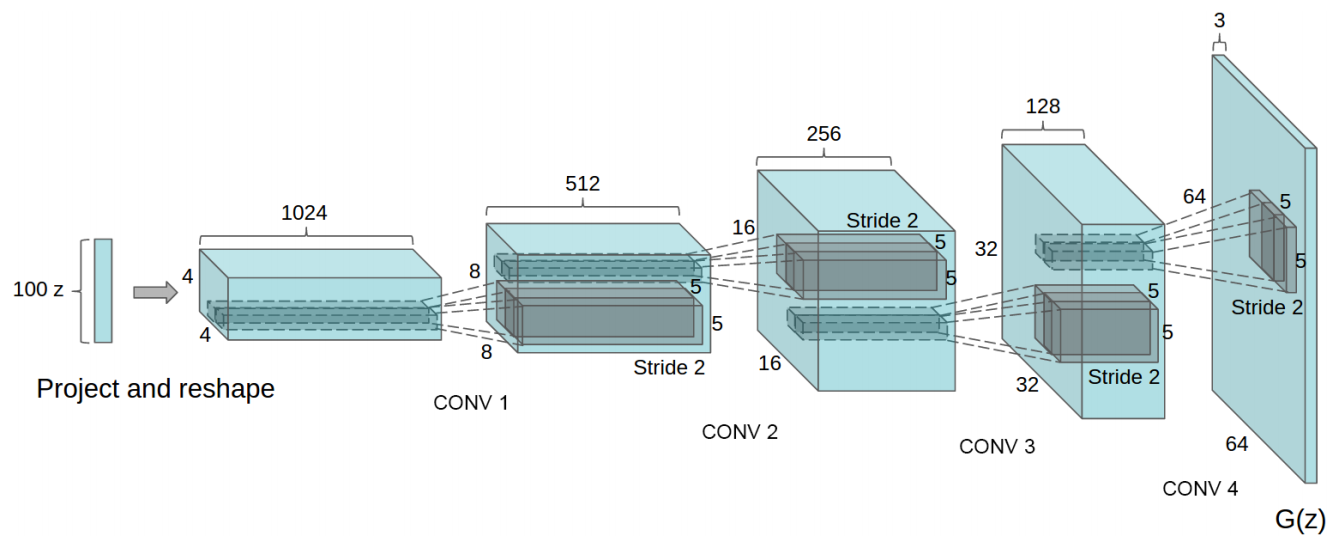
Next, we first define the generator model. According to the structure of DCGAN, the generator network will use transposed convolutional layers. Here we use torch.nn.ConvTranspose2d provided by PyTorch 🔗.

Exercise 65.1

Challenge: Define the generator network as required.

Requirement: During training, the input noise channel of the generator is 100. After passing through 5 transposed convolutional layers in sequence, it finally outputs a 3-channel tensor. The specific structure is as follows:

• In the transposed convolutional layers, except for the first transposed convolutional layer where stride and padding use the default parameters, for the remaining layers, stride = 2 and padding = 1. Additionally, for all transposed convolutional layers, kernel_size = 4, and no bias term is added. All other parameters use the default values.

• Batch normalization can use the BatchNorm2d() class. The shape of the input tensor is the same as that of the previous layer, and all other parameters use the default values. Official Documentation

## 补充代码 ###

Solution to Exercise 65.1

from torch import nn

class Generator(nn.Module):
    def __init__(self):
        super(Generator, self).__init__()
        self.main = nn.Sequential(
            # input is Z, going into a convolution
            nn.ConvTranspose2d( 100, 64 * 8, 4, 1, 0, bias=False),
            nn.BatchNorm2d(64 * 8),
            nn.ReLU(True),
            # state size. (64*8) x 4 x 4
            nn.ConvTranspose2d(64 * 8, 64 * 4, 4, 2, 1, bias=False),
            nn.BatchNorm2d(64 * 4),
            nn.ReLU(True),
            # state size. (64*4) x 8 x 8
            nn.ConvTranspose2d( 64 * 4, 64 * 2, 4, 2, 1, bias=False),
            nn.BatchNorm2d(64 * 2),
            nn.ReLU(True),
            # state size. (64*2) x 16 x 16
            nn.ConvTranspose2d( 64 * 2, 64, 4, 2, 1, bias=False),
            nn.BatchNorm2d(64),
            nn.ReLU(True),
            # state size. (64) x 32 x 32
            nn.ConvTranspose2d( 64, 3, 4, 2, 1, bias=False),
            nn.Tanh()
            # state size. (3) x 64 x 64
        )

    def forward(self, input):
        return self.main(input)

Run the test

Generator()

Expected output:

Generator(
  (main): Sequential(
    (0): ConvTranspose2d(100, 512, kernel_size=(4, 4), stride=(1, 1), bias=False)
    (1): BatchNorm2d(512, eps=1e-05, momentum=0.1, affine=True, track_running_stats=True)
    (2): ReLU(inplace)
    (3): ConvTranspose2d(512, 256, kernel_size=(4, 4), stride=(2, 2), padding=(1, 1), bias=False)
    (4): BatchNorm2d(256, eps=1e-05, momentum=0.1, affine=True, track_running_stats=True)
    (5): ReLU(inplace)
    (6): ConvTranspose2d(256, 128, kernel_size=(4, 4), stride=(2, 2), padding=(1, 1), bias=False)
    (7): BatchNorm2d(128, eps=1e-05, momentum=0.1, affine=True, track_running_stats=True)
    (8): ReLU(inplace)
    (9): ConvTranspose2d(128, 64, kernel_size=(4, 4), stride=(2, 2), padding=(1, 1), bias=False)
    (10): BatchNorm2d(64, eps=1e-05, momentum=0.1, affine=True, track_running_stats=True)
    (11): ReLU(inplace)
    (12): ConvTranspose2d(64, 3, kernel_size=(4, 4), stride=(2, 2), padding=(1, 1), bias=False)
    (13): Tanh()
  )
)

Next, we define the discriminator model.

Exercise 65.2

Challenge: Define the discriminator network as required.

Requirement: During training, the input image tensor to the discriminator has 3 channels. After passing through 5 convolutional layers in sequence, it finally outputs a 1D tensor to determine whether it meets the requirements. The specific structure is as follows:

• In the convolutional layers, except for the last convolutional layer where stride and padding use the default parameters, for the other layers, stride = 2 and padding = 1. Additionally, for all convolutional layers, kernel_size = 4, and no bias term is added. All other parameters use the default values.

• For batch normalization, the BatchNorm2d() class can be used. The shape of the input tensor is the same as that of the previous layer, and all other parameters use the default values. Official Documentation

• The activation function uses the variant of ReLU, LeakyReLU, with parameters negative_slope = 0.2 and inplace = True. Official Documentation

## 补充代码 ###

Solution to Exercise 65.2

class Discriminator(nn.Module):
    def __init__(self):
        super(Discriminator, self).__init__()
        self.main = nn.Sequential(
            # input is (3) x 64 x 64
            nn.Conv2d(3, 64, 4, 2, 1, bias=False),
            nn.BatchNorm2d(64),
            nn.LeakyReLU(0.2, inplace=True),
            # state size. (64) x 32 x 32
            nn.Conv2d(64, 64 * 2, 4, 2, 1, bias=False),
            nn.BatchNorm2d(64 * 2),
            nn.LeakyReLU(0.2, inplace=True),
            # state size. (64*2) x 16 x 16
            nn.Conv2d(64 * 2, 64 * 4, 4, 2, 1, bias=False),
            nn.BatchNorm2d(64 * 4),
            nn.LeakyReLU(0.2, inplace=True),
            # state size. (64*4) x 8 x 8
            nn.Conv2d(64 * 4, 64 * 8, 4, 2, 1, bias=False),
            nn.BatchNorm2d(64 * 8),
            nn.LeakyReLU(0.2, inplace=True),
            # state size. (64*8) x 4 x 4
            nn.Conv2d(64 * 8, 1, 4, 1, 0, bias=False),
            nn.Sigmoid()
        )

    def forward(self, input):
        return self.main(input)

Run the test

Discriminator()

Expected output:

Discriminator(
  (main): Sequential(
    (0): Conv2d(3, 64, kernel_size=(4, 4), stride=(2, 2), padding=(1, 1), bias=False)
    (1): BatchNorm2d(64, eps=1e-05, momentum=0.1, affine=True, track_running_stats=True)
    (2): LeakyReLU(negative_slope=0.2, inplace)
    (3): Conv2d(64, 128, kernel_size=(4, 4), stride=(2, 2), padding=(1, 1), bias=False)
    (4): BatchNorm2d(128, eps=1e-05, momentum=0.1, affine=True, track_running_stats=True)
    (5): LeakyReLU(negative_slope=0.2, inplace)
    (6): Conv2d(128, 256, kernel_size=(4, 4), stride=(2, 2), padding=(1, 1), bias=False)
    (7): BatchNorm2d(256, eps=1e-05, momentum=0.1, affine=True, track_running_stats=True)
    (8): LeakyReLU(negative_slope=0.2, inplace)
    (9): Conv2d(256, 512, kernel_size=(4, 4), stride=(2, 2), padding=(1, 1), bias=False)
    (10): BatchNorm2d(512, eps=1e-05, momentum=0.1, affine=True, track_running_stats=True)
    (11): LeakyReLU(negative_slope=0.2, inplace)
    (12): Conv2d(512, 1, kernel_size=(4, 4), stride=(1, 1), bias=False)
    (13): Sigmoid()
  )
)

After the network is built, the loss function, optimizer, etc. required for training need to be defined next.

# 如果 GPU 可用则使用 CUDA 加速，否则使用 CPU 设备计算
dev = torch.device("cuda") if torch.cuda.is_available() else torch.device("cpu")
dev

This experiment can be completed on a high - configuration CPU cloud host without using a GPU.

netD = Discriminator().to(dev)
netG = Generator().to(dev)
criterion = nn.BCELoss().to(dev)

lr = 0.0002  # 学习率
optimizerD = torch.optim.Adam(netD.parameters(), lr=lr, betas=(0.5, 0.999))  # Adam 优化器
optimizerG = torch.optim.Adam(netG.parameters(), lr=lr, betas=(0.5, 0.999))

Everything is ready, and it’s time to start training the model. The code challenges for training the model have been provided in full.

from torchvision.utils import make_grid
from matplotlib import pyplot as plt
from IPython import display

%matplotlib inline

epochs = 100
for epoch in range(epochs):
    for n, (images, _) in enumerate(dataloader):
        real_labels = torch.ones(images.size(0)).to(dev)  # 真实数据的标签为 1
        fake_labels = torch.zeros(images.size(0)).to(dev)  # 伪造数据的标签为 0

        # 使用真实图片训练判别器网络
        netD.zero_grad()  # 梯度置零
        output = netD(images.to(dev))  # 输入真实数据
        lossD_real = criterion(output.squeeze(), real_labels)  # 计算损失

        # 使用伪造图片训练判别器网络
        noise = torch.randn(images.size(0), 100, 1, 1).to(dev)  # 随机噪声，生成器输入
        fake_images = netG(noise)  # 通过生成器得到输出
        output2 = netD(fake_images.detach())  # 输入伪造数据
        lossD_fake = criterion(output2.squeeze(), fake_labels)  # 计算损失
        lossD = lossD_real + lossD_fake
        lossD.backward()
        optimizerD.step()

        # 训练生成器网络
        netG.zero_grad()
        output3 = netD(fake_images)
        lossG = criterion(output3.squeeze(), real_labels)
        lossG.backward()
        optimizerG.step()

        # 生成 64 组测试噪声样本，最终绘制 8x8 测试网格图像
        fixed_noise = torch.randn(64, 100, 1, 1).to(dev)
        fixed_images = netG(fixed_noise)
        fixed_images = make_grid(fixed_images.data, nrow=8, normalize=True).cpu()
        plt.figure(figsize=(6, 6))
        plt.title(
            "Epoch[{}/{}], Batch[{}/{}]".format(
                epoch + 1, epochs, n + 1, len(dataloader)
            )
        )
        plt.imshow(fixed_images.permute(1, 2, 0).numpy())
        display.display(plt.gcf())
        display.clear_output(wait=True)

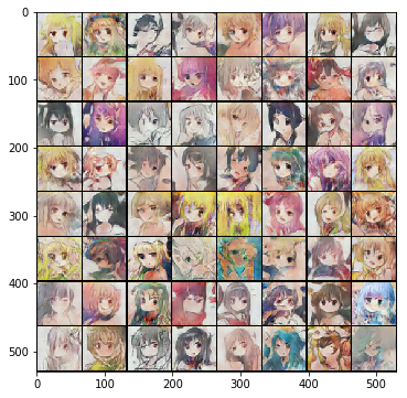
The training process of DCGAN is relatively slow. As the number of iterations increases, the effect gets better and better. After our tests, dozens of Epochs can already achieve a fairly good effect.

If you want to obtain more refined images, you may need to rely on higher - resolution datasets. For the practical content of using GAN to generate anime avatars, you can also refer to more open - source projects: jayleicn/animeGAN

---

○ Sharethis article link to your social media, blog, forum, etc. More external links will increase the search engine ranking of this site.

If you find this content helpful, you can buy me a coffee

Previous

64. Principle and Construction of Generative Adversarial Networks

Next

66. Autoencoder Principle and Construction