Pro Membership

Pro Membership is a membership plan created by the author to maintain and update this tutorial. You can get more benefits and services, click to view details.

43. Machine Learning Model Inference and Deployment#

43.1. Introduction#

Machine learning engineering uses locally trained models for inference and deploys them to the cloud when necessary. In this experiment, you will learn how to save, deploy, and infer models built with scikit-learn.

43.2. Key Points#

Model saving
Model deployment
Model inference

So far, I believe you are very familiar with the machine learning process. Generally, we use training data to build a model and then use validation data or test data to evaluate the model. In fact, the process of evaluating the model was also called prediction and evaluation earlier.

43.3. Model Inference#

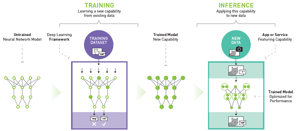
In fact, using a trained model to make predictions on new data has a more professional term in machine learning engineering called “Inference”. The following figure details the processes of neural network model training and inference. Making predictions on new input data through a neural network constructed with a training set is inference.

https://cdn.aibydoing.com/aibydoing/images/document-uid214893labid7506timestamp1553237955368.png

Source

Generally, inference is further divided into: static inference and dynamic inference.

Static inference is easy to understand. We perform inference on a batch of data centrally and store the results in a data table or database. When needed, we can directly obtain the inference results by querying.

Dynamic inference generally means that we deploy the model to a server. When needed, we send a request to the server to obtain the prediction results returned by the model. Different from static inference, the process of dynamic inference is calculated in real time, while static inference is processed in batches in advance.

Of course, both static and dynamic inference have their own advantages and disadvantages. Static inference is suitable for processing a large volume of data because dynamic inference is very time-consuming when dealing with a large amount of data. However, static inference cannot be updated in real time, while the results of dynamic inference are immediate calculation results.

I believe everyone is familiar with static inference because, in the previous content, our prediction of new data is actually similar to the process of static inference. You only need to use the predict operation provided by scikit-learn to complete it. Next, we will focus on the process of dynamic inference and teach you how to deploy a scikit-learn model and complete dynamic inference in the way of RESTful API.

43.4. Model Deployment#

To deploy a scikit-learn model, of course, you need to complete model training first.

Next, we train a Titanic survival inference model. The dataset is loaded through seaborn and previewed.

                          from seaborn import load_dataset
import pandas as pd
import numpy as np
import warnings

warnings.filterwarnings("ignore")  # 忽略模块变动警告

df = load_dataset("titanic")  # 加载泰坦尼克数据集
df

                        

	survived	pclass	sex	age	sibsp	parch	fare	embarked	class	who	adult_male	deck	embark_town	alive	alone
0	0	3	male	22.0	1	0	7.2500	S	Third	man	True	NaN	Southampton	no	False
1	1	1	female	38.0	1	0	71.2833	C	First	woman	False	C	Cherbourg	yes	False
2	1	3	female	26.0	0	0	7.9250	S	Third	woman	False	NaN	Southampton	yes	True
3	1	1	female	35.0	1	0	53.1000	S	First	woman	False	C	Southampton	yes	False
4	0	3	male	35.0	0	0	8.0500	S	Third	man	True	NaN	Southampton	no	True
...	...	...	...	...	...	...	...	...	...	...	...	...	...	...	...
886	0	2	male	27.0	0	0	13.0000	S	Second	man	True	NaN	Southampton	no	True
887	1	1	female	19.0	0	0	30.0000	S	First	woman	False	B	Southampton	yes	True
888	0	3	female	NaN	1	2	23.4500	S	Third	woman	False	NaN	Southampton	no	False
889	1	1	male	26.0	0	0	30.0000	C	First	man	True	C	Cherbourg	yes	True
890	0	3	male	32.0	0	0	7.7500	Q	Third	man	True	NaN	Queenstown	no	True

891 rows × 15 columns

As can be seen, the dataset contains a total of 15 columns and 891 samples. We select three features: the passenger class pclass, gender sex, and embarkation port embarked, and use whether the passenger is alive or not (alive) as the target value.

                          X = df[["pclass", "sex", "embarked"]]  # 特征
y = df["alive"]  # 目标

Before training, we first perform one-hot encoding on the feature data. The method of one-hot encoding has been introduced before.

                          X = pd.get_dummies(X)  # 独热编码
X.head()

	pclass	sex_female	sex_male	embarked_C	embarked_Q	embarked_S
0	3	False	True	False	False	True
1	1	True	False	True	False	False
2	3	True	False	False	False	True
3	1	True	False	False	False	True
4	3	False	True	False	False	True

Next, we can start training. Here, we use the random forest method to build a model and use cross-validation to evaluate the performance of the model.

                          from sklearn.model_selection import cross_val_score
from sklearn.ensemble import RandomForestClassifier

model = RandomForestClassifier()  # 随机森林
np.mean(cross_val_score(model, X, y, cv=5))  # 5 次交叉验证求平均

0.8114556525014125

Cross-validation shows that the classification accuracy of the model is approximately 81%.

To facilitate the deployment of the model, we need to store the trained model. Here, we can use sklearn.externals.joblib provided by scikit-learn to save the model as a .pkl binary file. The method of saving the model is very simple. Just read the following code.

                          import joblib

model.fit(X, y)  # 训练模型
joblib.dump(model, "titanic.pkl")  # 保存模型

['titanic.pkl']

Now that we have the model file, we can deploy the model. We plan to deploy the model to the cloud (for local testing), and here we use Flask to achieve this. Flask is a well-known Python web application framework that can be used to build a RESTful API. Since the content of Flask is not covered in this course, you need to understand the following code by yourself in combination with the official documentation.

                          %writefile predict.py
from flask import Flask, request, jsonify
import joblib
import pandas as pd

app = Flask(__name__)


@app.route("/", methods=["POST"])  # 请求方法为 POST
def predict():
    json_ = request.json  # 解析请求数据
    query_df = pd.DataFrame(json_)  # 将 JSON 变为 DataFrame
    columns_onehot = [
        "pclass",
        "sex_female",
        "sex_male",
        "embarked_C",
        "embarked_Q",
        "embarked_S",
    ]  # 独热编码 DataFrame 列名
    query = pd.get_dummies(query_df).reindex(
        columns=columns_onehot, fill_value=0
    )  # 将请求数据 DataFrame 处理成独热编码样式
    clf = joblib.load("titanic.pkl")  # 加载模型
    prediction = clf.predict(query)  # 模型推理
    return jsonify({"prediction": list(prediction)})  # 返回推理结果

                        

Overwriting predict.py

First, execute predict.py in the terminal to start the Flask app.

                      $ python predict.py

* Serving Flask app "predict" (lazy loading)
* Environment: production
WARNING: Do not use the development server in a production environment.
Use a production WSGI server instead.
* Debug mode: off
* Running on http://127.0.0.1:5000/ (Press CTRL+C to quit)

                    

Open a new terminal to send requests to the destination address.

                      In [1]: import requests                                                                             

In [2]: sample = [{"pclass": 1, "sex": "male", "embarked": "C"}, {"pclass": 2, "sex": "female", "embarked": "S"}]                             
In [3]: requests.post(url='http://127.0.0.1:5000', json=sample).content                             
Out[3]: b'{"prediction":["no","yes"]}\n'

Here, we provide the test address of the experimental example model deployed in the cloud: https://titanic-demo.onrender.com, and you can directly obtain the test results:

                          import requests

# 向服务器发送请求获得预测结果
sample = [
    {"pclass": 1, "sex": "male", "embarked": "C"},
    {"pclass": 2, "sex": "female", "embarked": "S"},
    {"pclass": 3, "sex": "male", "embarked": "Q"},
    {"pclass": 3, "sex": "female", "embarked": "S"},
]

# 稍等片刻，Render 线上服务存在冷却启动时间
requests.post(url="https://titanic-demo.onrender.com", json=sample).content

                        

b'{"predict":["no","yes","no","no"]}\n'

You can read and refer to the source code of this project.

43.5. Summary#

In this course, we learned about the saving, deployment, and dynamic inference of scikit-learn models. Since the use of Flask is involved, some knowledge needs to be supplemented by the students themselves. However, I believe you have been able to understand the complete process from the content of the experiment. In fact, with the development of cloud technology, it has become more convenient to deploy models online. Similar to the cloud functions launched by Google Cloud or the AWS Lambda function, machine learning models can be quickly deployed without a server. If you are interested, you can search and learn by yourself.

○ Sharethis article link to your social media, blog, forum, etc. More external links will increase the search engine ranking of this site.

If you find this content helpful, you can buy me a coffee

42. Handwritten Character Classification with AutoML

44. Mushroom Classification Model Deployment and Inference