Pro Membership

Pro Membership is a membership plan created by the author to maintain and update this tutorial. You can get more benefits and services, click to view details.

20. Decision Tree Implementation and Application#

20.1. Introduction#

Decision tree is a simple and classic algorithm in machine learning. This experiment will guide you to learn the principle of decision tree, understand the feature selection of decision classification in detail through code, implement the algorithm process of decision tree through Python, learn to build a decision tree model using scikit-learn, and finally use this model to classify and predict real data.

20.2. Key Points#

Principle of Decision Tree Algorithm
Information Gain
Implementation of Decision Tree Algorithm
Classification Prediction of Student Grades
Visualization of Decision Tree

20.3. What is a Decision Tree#

A decision tree is a special tree structure, generally composed of nodes and directed edges. Among them, nodes represent features, attributes, or a class, while directed edges contain judgment conditions. The decision tree starts from the root node and extends. After passing through different judgment conditions, it reaches different child nodes. And the upper-level child nodes can be further divided into lower-level child nodes as parent nodes. Generally, we input data from the root node. After multiple judgments, this data will be classified into different categories. This constitutes a simple classification decision tree.

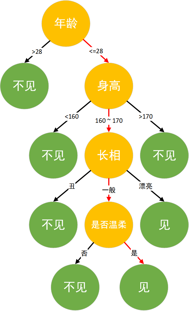
For a popular example, suppose there is a conversation between Xiaolou, who has been single for many years after working, and his mother when she is introducing blind dates to him:

Mother: Xiaolou, you’re already 28 and still single. There will be a girl from a relative’s family coming tomorrow. Do you want to go and meet her? Xiaolou: How old is she? Mother: 26. Xiaolou: How tall is she? Mother: 165 centimeters. Xiaolou: Is she good-looking? Mother: She’s okay. She’s quite plain. Xiaolou: Is she gentle? Mother: She seems quite gentle and very polite. Xiaolou: Okay, I’ll go and meet her.

Xiaolou, as a programmer, his thinking logic is a typical decision tree classification logic. He takes age, height, appearance, and gentleness as features and finally makes a decision on whether to meet or not. The decision logic is shown in the figure:

https://cdn.aibydoing.com/aibydoing/images/document-uid214893labid6671timestamp1531711818867.png

20.4. Principle of Decision Tree Algorithm#

In fact, the decision tree algorithm is just like the above scenario, and its idea is very easy to understand. The specific algorithm process is as follows:

Data Preparation → Through data cleaning and data processing, organize the data into a vector without missing values.
Find the Best Feature → Traverse each partitioning method of each feature to find the best partitioning feature.
Generate Branches → Divide into two or more nodes.
Generate a Decision Tree → For the split nodes, continue to execute steps 2 - 3 respectively until each node has only one category.
Decision Classification → According to the trained decision tree model, classify the prediction data.

Next, we will implement the construction and classification of a decision tree in Python according to the algorithm process of the decision tree. First, generate a set of data. The data contains two categories, man and woman, and the features are: hair (length of hair), voice (thickness of voice), height (height), and ear_stud (whether wearing stud earrings).

                          import numpy as np
import pandas as pd


def create_data():
    # 生成示例数据
    data_value = np.array(
        [
            ["long", "thick", 175, "no", "man"],
            ["short", "medium", 168, "no", "man"],
            ["short", "thin", 178, "yes", "man"],
            ["short", "thick", 172, "no", "man"],
            ["long", "medium", 163, "no", "man"],
            ["short", "thick", 180, "no", "man"],
            ["long", "thick", 173, "yes", "man"],
            ["short", "thin", 174, "no", "man"],
            ["long", "thin", 164, "yes", "woman"],
            ["long", "medium", 158, "yes", "woman"],
            ["long", "thick", 161, "yes", "woman"],
            ["short", "thin", 166, "yes", "woman"],
            ["long", "thin", 158, "no", "woman"],
            ["short", "medium", 163, "no", "woman"],
            ["long", "thick", 161, "yes", "woman"],
            ["long", "thin", 164, "no", "woman"],
            ["short", "medium", 172, "yes", "woman"],
        ]
    )
    columns = np.array(["hair", "voice", "height", "ear_stud", "labels"])
    data = pd.DataFrame(data_value.reshape(17, 5), columns=columns)
    return data

                        

After creating the data, load and print out this data.

                          data = create_data()
data

	hair	voice	height	ear_stud	labels
0	long	thick	175	no	man
1	short	medium	168	no	man
2	short	thin	178	yes	man
3	short	thick	172	no	man
4	long	medium	163	no	man
5	short	thick	180	no	man
6	long	thick	173	yes	man
7	short	thin	174	no	man
8	long	thin	164	yes	woman
9	long	medium	158	yes	woman
10	long	thick	161	yes	woman
11	short	thin	166	yes	woman
12	long	thin	158	no	woman
13	short	medium	163	no	woman
14	long	thick	161	yes	woman
15	long	thin	164	no	woman
16	short	medium	172	yes	woman

After obtaining the data, according to the algorithm process, the next step is to find the optimal partitioning feature. As the partitioning progresses, we try our best to classify the samples contained in the partitioning branches into the same category, that is, the “purity” of the nodes becomes higher and higher. The commonly used feature partitioning methods are information gain and gain ratio.

20.5. Information Gain (ID3)#

Before introducing information gain, the concept of “information entropy” is introduced first. Information entropy is one of the most commonly used metrics to measure the purity of samples, and its formula is:

\[ \operatorname{Ent}(\operatorname{D})=-\sum_{k=1}^{\left |y \right |}p_{k}\; log_{2}p_{k} \tag{1} \]

Among them, \(\operatorname{D}\) represents the sample set, and \(p_{k}\) represents the proportion of samples in the \(k\)-th class. The smaller the value of \(\operatorname{Ent}(\operatorname{D})\), the higher the purity of \(\operatorname{D}\). According to the above data, when calculating the information entropy of the data set, \(\left | y \right |\) obviously has only 2 types, namely man and woman. Among them, the probability of man is \(\frac{8}{17}\), and the probability of woman is \(\frac{9}{17}\). Then, according to formula \((1)\), the purity of the data set is obtained as:

\[ \operatorname{Ent}(\operatorname{data})=-\sum_{k=1}^{2}p_{k}\;log_{2}p_{k}=-(\frac{8}{17}log_{2}\frac{8}{17}+\frac{9}{17}log_{2}\frac{9}{17})=0.9975 \]

Next, define a function to calculate information entropy.

                          import math


def get_Ent(data):
    """
    参数:
    data -- 数据集

    返回:
    Ent -- 信息熵
    """
    # 计算信息熵
    num_sample = len(data)  # 样本个数
    label_counts = {}  # 初始化标签统计字典
    for i in range(num_sample):
        each_data = data.iloc[i, :]
        current_label = each_data["labels"]  # 得到当前元素的标签（label）

        # 如果标签不在当前字典中，添加该类标签并初始化 value=0,否则该类标签 value+1
        if current_label not in label_counts.keys():
            label_counts[current_label] = 0
        label_counts[current_label] += 1

    Ent = 0.0  # 初始化信息熵
    for key in label_counts:
        prob = float(label_counts[key]) / num_sample
        Ent -= prob * math.log(prob, 2)  # 应用信息熵公式计算信息熵
    return Ent

                        

Calculate the information entropy of the root node by using the information entropy calculation function:

                          base_ent = get_Ent(data)
base_ent

0.9975025463691153

Information gain is based on information entropy. For a discrete feature \(x\) with \(M\) values, if we use \(x\) to partition the sample set \(\operatorname{D}\), it will generate \(M\) branches. The \(m\)-th branch contains all samples in \(\operatorname{D}\) with the value \(m\) on the feature \(x\), denoted as \(\operatorname{D}^{m}\) (for example: according to the data generated above, if we partition by hair, it will generate two branches, long and short, and each branch contains the data in the whole set that belongs to long or short respectively).

Considering that different branch nodes contain different numbers of samples, we assign a weight \(\frac{\left | \operatorname{D}^{m}\right |}{\left | \operatorname{D} \right |}\) to each branch so that the branch node with more samples has a greater impact. Then the formula for information gain can be obtained as follows:

\[ \operatorname{Gain}(\operatorname{D},x)=\operatorname{Ent}(\operatorname{D})- \sum_{m=1}^{M}\frac{\left | \operatorname{D}^{m}\right |}{\left | \operatorname{D} \right |}\operatorname{Ent}(\operatorname{D}^{m}) \tag{2} \]

Generally, the larger the information gain, the higher the purity of using \(x\) to partition the sample set \(\operatorname{D}\). Taking hair as an example, it has two possible values, short and long, which are represented by \(\operatorname{D}^{1}\) (hair = long) and \(\operatorname{D}^{2}\) (hair = short) respectively.

Among them, the data numbers of \(\operatorname{D}^{1}\) are \(\{0, 4, 6, 8, 9, 10, 12, 14, 15\}\), a total of 9. Among these, there are \(\{0, 4, 6\}\), a total of 3 men, accounting for \(\frac{3}{9}\), and \(\{8, 9, 10, 12, 14, 15\}\), a total of 6 women, accounting for \(\frac{6}{9}\).

Similarly, the numbers of \(\operatorname{D}^{2}\) are \(\{1, 2, 3, 5, 7, 11, 13, 16\}\), a total of 8. Among them, there are \(\{1, 2, 3, 5, 7\}\), a total of 5 men, accounting for \(\frac{5}{8}\), and \(\{11, 13, 16\}\), a total of 3 women, accounting for \(\frac{3}{8}\). If we partition according to hair, the information entropy of the two branch nodes is:

\[\operatorname{Ent}(\operatorname{D}^{1})=-(\frac{3}{9}\;log_{2}\frac{3}{9}+\frac{6}{9}\;log_{2}\frac{6}{9})=0.449\]

\[\operatorname{Ent}(\operatorname{D}^{2})=-(\frac{5}{8}\;log_{2}\frac{5}{8}+\frac{3}{8}\;log_{2}\frac{3}{8})=0.486\]

According to the formula of information gain, the information gain of hair can be calculated as:

\[ \operatorname{Gain}(\operatorname{D}, \text {hair})=\operatorname{Ent}(\operatorname{D})-\sum_{m=1}^{2} \frac{\left|\operatorname{D}^{m}\right|}{|\operatorname{D}|} \operatorname{Ent}\left(\operatorname{D}^{m}\right)=0.9975-\left(\frac{9}{17} * 0.449+\frac{8}{17} * 0.486\right)=0.062 \]

Next, we use Python to implement the information gain (ID3) algorithm:

                          def get_gain(data, base_ent, feature):
    """
    参数:
    data -- 数据集
    base_ent -- 根节点的信息熵
    feature -- 计算信息增益的特征

    返回:
    Ent -- 信息熵
    """
    # 计算信息增益
    feature_list = data[feature]  # 得到一个特征的全部取值
    unique_value = set(feature_list)  # 特征取值的类别
    feature_ent = 0.0

    for each_feature in unique_value:
        temp_data = data[data[feature] == each_feature]
        weight = len(temp_data) / len(feature_list)  # 计算该特征的权重值
        temp_ent = weight * get_Ent(temp_data)
        feature_ent = feature_ent + temp_ent

    gain = base_ent - feature_ent  # 信息增益
    return gain

                        

After completing the information gain function, try to calculate the information gain value of the feature hair.

                          get_gain(data, base_ent, "hair")

                        

0.062200515199107964

20.6. Information Gain Ratio (C4.5)#

There are also many deficiencies in information gain. Through a large number of experiments, it is found that when information gain is used as the criterion, it is prone to bias towards features with more values. To avoid the adverse effects of this preference on the prediction results, the gain ratio can be used to select the optimal partition. The formula for the gain ratio is defined as:

\[ \operatorname{GainRatio}(\operatorname{D},a)=\frac{\operatorname{Gain}(\operatorname{D},a)}{\operatorname{IV}(a)} \tag{3} \]

where:

\[ \operatorname{IV}(a)=-\sum_{m=1}^{M}\frac{\left | \operatorname{D}^{m} \right |}{\left | \operatorname{D} \right |}\; log_{2}\frac{\left | \operatorname{D}^{m} \right |}{\left | \operatorname{D} \right |} \tag{4} \]

\(\operatorname{IV}(a)\) is called the intrinsic value of feature \(a\). When the number of values of \(a\) is larger, the value of \(\operatorname{IV}(a)\) is usually relatively large. For example:

\[\operatorname{IV}(\operatorname{hair})= -\frac{9}{17}\; log_{2}\frac{9}{17}-\frac{8}{17}\; log_{2}\frac{8}{17}=0.998 \]

\[\operatorname{IV}(\operatorname{voice})= -\frac{7}{17}\; log_{2}\frac{7}{17} -\frac{5}{17}\; log_{2}\frac{5}{17} - \frac{5}{17}\; log_{2}\frac{5}{17} = 1.566\]

20.7. Continuous Value Processing#

In the feature selection introduced above, discrete data is processed. However, in real life, continuous values often appear in data, such as height in the generated data. When the data is small, each value can be regarded as a category. But when the data volume is large, this is not advisable. In the C4.5 algorithm, the dichotomy method is used to process continuous values.

For a continuous attribute \(X\), assume that there are \(n\) different values in total. Sort these values in ascending order as \(\{x_{1},x_{2},x_{3},…,x_{n} \}\). Then find a point \(t\) as the splitting point. The data will be divided into two categories, one with values greater than \(t\) and the other with values less than \(t\). Usually, the value of \(t\) is the average of two adjacent points, \(t=\frac{x_{i}+x_{i+1}}{2}\).

Among the \(n\) continuous values, there are \(n - 1\) possible values for \(t\) that can serve as splitting points. By traversing, these splitting points can be examined in the same way as discrete data.

\[ \operatorname{Gain}(\operatorname{D}, X)=\operatorname{Ent}(\operatorname{D})-\frac{\left|\operatorname{D}<t\right|}{|\operatorname{D}|} \operatorname{Ent}\left(\operatorname{D}<t\right)-\frac{\left|\operatorname{D}>t\right|}{|\operatorname{D}|} \operatorname{Ent}\left(\operatorname{D}>t\right) \tag{5} \]

Among them, the information gain after dichotomizing the sample \(\operatorname{D}\) based on the splitting point \(t\) is obtained. Then we can select the splitting point that maximizes the value of \(\operatorname{Gain}(\operatorname{D},X)\).

                          def get_splitpoint(data, base_ent, feature):
    """
    参数:
    data -- 数据集
    base_ent -- 根节点的信息熵
    feature -- 需要划分的连续特征

    返回:
    final_t -- 连续值最优划分点
    """
    # 将连续值进行排序并转化为浮点类型
    continues_value = data[feature].sort_values().astype(np.float64)
    continues_value = [i for i in continues_value]  # 不保留原来的索引
    t_set = []
    t_ent = {}

    # 得到划分点 t 的集合
    for i in range(len(continues_value) - 1):
        temp_t = (continues_value[i] + continues_value[i + 1]) / 2
        t_set.append(temp_t)

    # 计算最优划分点
    for each_t in t_set:
        # 将大于划分点的分为一类
        temp1_data = data[data[feature].astype(np.float64) > each_t]
        # 将小于划分点的分为一类
        temp2_data = data[data[feature].astype(np.float64) < each_t]
        weight1 = len(temp1_data) / len(data)
        weight2 = len(temp2_data) / len(data)
        # 计算每个划分点的信息增益
        temp_ent = (
            base_ent - weight1 * get_Ent(temp1_data) - weight2 * get_Ent(temp2_data)
        )
        t_ent[each_t] = temp_ent
    print("t_ent:", t_ent)
    final_t = max(t_ent, key=t_ent.get)
    return final_t

                        

After implementing the function for the optimal splitting point of continuous values, find the splitting points for the continuous eigenvalues of height.

                          final_t = get_splitpoint(data, base_ent, "height")
final_t

                          t_ent: {158.0: 0.1179805181500242, 159.5: 0.1179805181500242, 161.0: 0.2624392604045631, 162.0: 0.2624392604045631, 163.0: 0.3856047022157598, 163.5: 0.15618502398692893, 164.0: 0.3635040117533678, 165.0: 0.33712865788827096, 167.0: 0.4752766311586692, 170.0: 0.32920899348970845, 172.0: 0.5728389611412551, 172.5: 0.4248356349861979, 173.5: 0.3165383509071513, 174.5: 0.22314940393447813, 176.5: 0.14078143361499595, 179.0: 0.06696192680347068}

                        

172.0

20.8. Decision Tree Algorithm Implementation#

After the best feature selection and continuous value processing in the decision tree, the next step is to construct the decision tree.

First, we process the continuous values. After finding the optimal splitting point, we set the values less than \(t\) to 0 and the values greater than or equal to \(t\) to 1.

                          def choice_1(x, t):
    if x > t:
        return ">{}".format(t)
    else:
        return "<{}".format(t)


deal_data = data.copy()
# 使用lambda和map函数将 height 按照final_t划分为两个类别
deal_data["height"] = pd.Series(
    map(lambda x: choice_1(int(x), final_t), deal_data["height"])
)
deal_data

                        

	hair	voice	height	ear_stud	labels
0	long	thick	>172.0	no	man
1	short	medium	<172.0	no	man
2	short	thin	>172.0	yes	man
3	short	thick	<172.0	no	man
4	long	medium	<172.0	no	man
5	short	thick	>172.0	no	man
6	long	thick	>172.0	yes	man
7	short	thin	>172.0	no	man
8	long	thin	<172.0	yes	woman
9	long	medium	<172.0	yes	woman
10	long	thick	<172.0	yes	woman
11	short	thin	<172.0	yes	woman
12	long	thin	<172.0	no	woman
13	short	medium	<172.0	no	woman
14	long	thick	<172.0	yes	woman
15	long	thin	<172.0	no	woman
16	short	medium	<172.0	yes	woman

After preprocessing the data, the next step is to select the optimal splitting feature.

                          def choose_feature(data):
    """
    参数:
    data -- 数据集

    返回:
    best_feature -- 最优的划分特征
    """
    # 选择最优划分特征
    num_features = len(data.columns) - 1  # 特征数量
    base_ent = get_Ent(data)
    best_gain = 0.0  # 初始化信息增益
    best_feature = data.columns[0]
    for i in range(num_features):  # 遍历所有特征
        temp_gain = get_gain(data, base_ent, data.columns[i])  # 计算信息增益
        if temp_gain > best_gain:  # 选择最大的信息增益
            best_gain = temp_gain
            best_feature = data.columns[i]
    return best_feature  # 返回最优特征

                        

After completing the function, let’s first see what the feature with the largest information gain value in the dataset is?

                          choose_feature(deal_data)

                        

'height'

After building all the sub - modules, the last step is to construct the core decision tree. In this experiment, the decision tree is constructed using the information gain (ID3) method. During the construction process, according to the algorithm flow, we repeatedly traverse the dataset, calculate the information gain of each feature, and through comparison, select the best feature as the parent node. Then, based on the values of the feature, we determine the branch child nodes. After that, we repeat the above operations until all the data in a certain branch belong to the same category, or we have traversed all the data features. When we reach the last feature, if the branch data is still “impure”, we take the category with the larger number as the child node.

Therefore, it is best to use a recursive approach to construct the decision tree.

                          def create_tree(data):
    """
    参数:
    data -- 数据集

    返回:
    tree -- 以字典的形式返回决策树
    """
    # 构建决策树
    feature_list = data.columns[:-1].tolist()
    label_list = data.iloc[:, -1]
    if len(data["labels"].value_counts()) == 1:
        leaf_node = data["labels"].mode().values
        return leaf_node  # 第一个递归结束条件：所有的类标签完全相同
    if len(feature_list) == 1:
        leaf_node = data["labels"].mode().values
        return leaf_node  # 第二个递归结束条件：用完了所有特征
    best_feature = choose_feature(data)  # 最优划分特征
    tree = {best_feature: {}}
    feat_values = data[best_feature]
    unique_value = set(feat_values)
    for value in unique_value:
        temp_data = data[data[best_feature] == value]
        temp_data = temp_data.drop([best_feature], axis=1)
        tree[best_feature][value] = create_tree(temp_data)
    return tree

                        

After completing the function to create the decision tree, the next step is to create our first tree.

                          tree = create_tree(deal_data)
tree

                          {'height': {'>172.0': array(['man'], dtype=object),
  '<172.0': {'ear_stud': {'yes': array(['woman'], dtype=object),
    'no': {'voice': {'thin': array(['woman'], dtype=object),
      'medium': array(['man'], dtype=object),
      'thick': array(['man'], dtype=object)}}}}}}

                        

The constructed tree can be represented in the form of a dictionary, and it can be understood more intuitively through images.

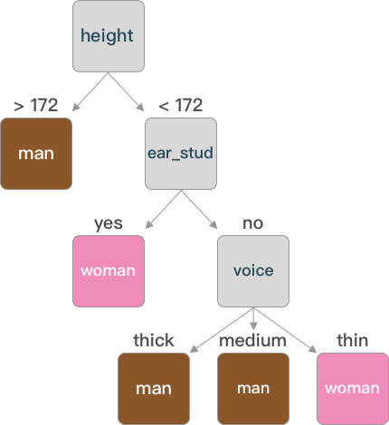
As can be seen from the graph, not every feature will necessarily become a node of the decision tree (such as “hair”) when constructing the decision tree.

After constructing the decision tree, it can finally be used to predict and classify unknown samples.

                          def classify(tree, test):
    """
    参数:
    data -- 数据集
    test -- 需要测试的数据

    返回:
    class_label -- 分类结果
    """
    # 决策分类
    first_feature = list(tree.keys())[0]  # 获取根节点
    feature_dict = tree[first_feature]  # 根节点下的树
    labels = test.columns.tolist()
    value = test[first_feature][0]
    for key in feature_dict.keys():
        if value == key:
            if type(feature_dict[key]).__name__ == "dict":  # 判断该节点是否为叶节点
                class_label = classify(feature_dict[key], test)  # 采用递归直到遍历到叶节点
            else:
                class_label = feature_dict[key]
    return class_label

                        

After the classification function is completed, next we try to classify the unknown data.

                          test = pd.DataFrame(
    {"hair": ["long"], "voice": ["thin"], "height": [163], "ear_stud": ["yes"]}
)
test

                        

	hair	voice	height	ear_stud
0	long	thin	163	yes

Preprocess continuous values:

                          test["height"] = pd.Series(map(lambda x: choice_1(int(x), final_t), test["height"]))
test

	hair	voice	height	ear_stud
0	long	thin	<172.0	yes

Classification prediction:

                          classify(tree, test)

                        

array(['woman'], dtype=object)

A person who is 163 centimeters tall, has long hair, wears stud earrings and has a slender voice is predicted to be a female after being judged by the decision tree we constructed.

In the above experiment, we did not consider the case of \(=\) splitting point. You can try to classify \(>=\) splitting point or \(<=\) splitting point into one category by yourself and see what differences there are in the results?

20.9. Pre - pruning and Post - pruning#

During the construction of a decision tree, especially when there are a large number of data features, in order to divide each training sample correctly as much as possible, the division of nodes will keep repeating, resulting in a large number of branches in a decision tree. For the training set, the fitted model is very perfect. However, this kind of perfection increases the complexity of the overall model and at the same time reduces the prediction ability for other data sets. That is to say, the overfitting we often mention makes the generalization ability of the model weaker. To avoid the occurrence of overfitting problems, the two most common methods in decision trees are pre - pruning and post - pruning.

20.10. Pre - pruning#

Pre - pruning, as the name implies, pre - cuts the branches and leaves. When constructing a decision tree model, an estimate is made before each data division. If the division of the current node does not bring an improvement in the generalization of the decision tree, the division is stopped and the current node is marked as a leaf node. For example, in the decision tree constructed earlier, according to the construction principle of the decision tree, after dividing by the height feature, the branch <172 is further divided according to the ear_stud feature value. If pre - pruning is applied, after dividing by the height feature, when deciding whether to divide the branch <172 by the ear_stud feature, calculate the accuracy before and after the division. If the accuracy after division is higher, continue to divide according to ear_stud; if it is lower, stop the division.

20.11. Post - pruning#

Different from pre - pruning which determines whether to continue feature division during the construction of a decision tree, post - pruning prunes the tree after the decision tree is constructed. If pre - pruning is a top - down pruning, then post - pruning is a bottom - up pruning. Post - pruning replaces the final branch node with a leaf node, and judges whether it brings an improvement in the generalization of the decision tree. If so, it performs pruning and replaces the branch node with a leaf node; otherwise, it does not perform pruning. For example, after the decision tree is constructed earlier, for the voice feature in the branch >172, replace it with a leaf node such as (man), calculate the division accuracy before and after the replacement. If the accuracy is higher after the replacement, perform pruning (replace the branch node with a leaf node); otherwise, do not prune.

20.12. Student Performance Classification Prediction#

Previously, we used Python to explain in detail the feature selection, continuous value processing, and prediction classification of decision trees. Next, we apply the decision tree model to classify and predict real data.

The data used in this application is the student performance dataset course-13-student.csv, which contains a total of 395 data entries and 26 features. First, load and preview the dataset:

                          wget -nc https://cdn.aibydoing.com/aibydoing/files/course-13-student.csv

                        

                          # 导入数据集并预览
stu_grade = pd.read_csv("course-13-student.csv")
stu_grade.head()

                        

	school	sex	address	Pstatus	Pedu	reason	guardian	traveltime	studytime	schoolsup	...	famrel	freetime	goout	Dalc	Walc	health	absences	G1	G2	G3
0	GP	F	U	A	4.0	course	mother	2	2	yes	...	4	3	4	1	1	3	6	5	6	6
1	GP	F	U	T	1.0	course	father	1	2	no	...	5	3	3	1	1	3	4	5	5	6
2	GP	F	U	T	1.0	other	mother	1	2	yes	...	4	3	2	2	3	3	10	7	8	10
3	GP	F	U	T	3.0	home	mother	1	3	no	...	3	2	2	1	1	5	2	15	14	15
4	GP	F	U	T	3.0	home	father	1	2	no	...	4	3	2	1	2	5	4	6	10	10

5 rows × 27 columns

Due to the excessive number of features, we select some features as the classification features for the decision tree model, which are:

school: The school the student attends (GP, MS)
sex: Gender (F: Female, M: Male)
address: Home address (U: Urban, R: Rural)
Pstatus: Parents’ status (A: Living together, T: Separated)
Pedu: Parents’ education level from low to high
reason: Reason for choosing this school (home: Family, course: Course design, reputation: School status, other: Others)
guardian: Guardian (mother: Mother, father: Father, other: Others)
studytime: Weekend study duration
schoolsup: Additional educational support (yes: Yes, no: No)
famsup: Family educational support (yes: Yes, no: No)
paid: Whether attending tutoring classes (yes: Yes, no: No)
higher: Whether wanting better education (yes: Yes, no: No)
internet: Whether having internet at home (yes: Yes, no: No)
G1: Test scores in the first stage
G2: Test scores in the second stage
G3: Final scores

                          new_data = stu_grade.iloc[:, [0, 1, 2, 3, 4, 5, 6, 8, 9, 10, 11, 14, 15, 24, 25, 26]]
new_data.head()

	school	sex	address	Pstatus	Pedu	reason	guardian	studytime	schoolsup	famsup	paid	higher	internet	G1	G2	G3
0	GP	F	U	A	4.0	course	mother	2	yes	no	no	yes	no	5	6	6
1	GP	F	U	T	1.0	course	father	2	no	yes	no	yes	yes	5	5	6
2	GP	F	U	T	1.0	other	mother	2	yes	no	yes	yes	yes	7	8	10
3	GP	F	U	T	3.0	home	mother	3	no	yes	yes	yes	yes	15	14	15
4	GP	F	U	T	3.0	home	father	2	no	yes	yes	yes	no	6	10	10

First, we classify the scores G1, G2, and G3 according to the scores. Scores from 0 to 4 are classified as bad, and scores from 5 to 9 are classified as medium.

                          def choice_2(x):
    x = int(x)
    if x < 5:
        return "bad"
    elif x >= 5 and x < 10:
        return "medium"
    elif x >= 10 and x < 15:
        return "good"
    else:
        return "excellent"


stu_data = new_data.copy()
stu_data["G1"] = pd.Series(map(lambda x: choice_2(x), stu_data["G1"]))
stu_data["G2"] = pd.Series(map(lambda x: choice_2(x), stu_data["G2"]))
stu_data["G3"] = pd.Series(map(lambda x: choice_2(x), stu_data["G3"]))
stu_data.head()

                        

	school	sex	address	Pstatus	Pedu	reason	guardian	studytime	schoolsup	famsup	paid	higher	internet	G1	G2	G3
0	GP	F	U	A	4.0	course	mother	2	yes	no	no	yes	no	medium	medium	medium
1	GP	F	U	T	1.0	course	father	2	no	yes	no	yes	yes	medium	medium	medium
2	GP	F	U	T	1.0	other	mother	2	yes	no	yes	yes	yes	medium	medium	good
3	GP	F	U	T	3.0	home	mother	3	no	yes	yes	yes	yes	excellent	good	excellent
4	GP	F	U	T	3.0	home	father	2	no	yes	yes	yes	no	medium	good	good

Similarly, we also classify Pedu (parents’ education level).

                          def choice_3(x):
    x = int(x)
    if x > 3:
        return "high"
    elif x > 1.5:
        return "medium"
    else:
        return "low"


stu_data["Pedu"] = pd.Series(map(lambda x: choice_3(x), stu_data["Pedu"]))
stu_data.head()

                        

	school	sex	address	Pstatus	Pedu	reason	guardian	studytime	schoolsup	famsup	paid	higher	internet	G1	G2	G3
0	GP	F	U	A	high	course	mother	2	yes	no	no	yes	no	medium	medium	medium
1	GP	F	U	T	low	course	father	2	no	yes	no	yes	yes	medium	medium	medium
2	GP	F	U	T	low	other	mother	2	yes	no	yes	yes	yes	medium	medium	good
3	GP	F	U	T	medium	home	mother	3	no	yes	yes	yes	yes	excellent	good	excellent
4	GP	F	U	T	medium	home	father	2	no	yes	yes	yes	no	medium	good	good

After the grade classification, to comply with the input specifications of scikit-learn functions, it is necessary to replace the data features.

                          def replace_feature(data):
    """
    参数:
    data -- 数据集

    返回:
    data -- 将特征值替换后的数据集
    """
    # 特征值替换
    for each in data.columns:  # 遍历每一个特征名称
        feature_list = data[each]
        unique_value = set(feature_list)
        i = 0
        for fea_value in unique_value:
            data[each] = data[each].replace(fea_value, i)
            i += 1
    return data

                        

After replacing the feature values, display them.

                          stu_data = replace_feature(stu_data)
stu_data.head()

	sex	Pstatus	Pedu	reason	guardian	studytime	schoolsup	famsup	paid	internet	G1	G2	G3
0	1	1	1	0	0	1	0	1	1	1	0	0	0
1	1	0	0	0	2	1	1	0	1	0	0	0	0
2	1	0	0	1	0	1	0	1	0	0	0	0	3
3	1	0	2	3	0	2	1	0	0	0	1	3	1
4	1	0	2	3	2	1	1	0	0	1	0	3	3

After loading the preprocessed dataset, in order to implement the decision tree algorithm, we also need to divide the dataset into a training set and a test set. According to experience, the training set accounts for 70% and the test set accounts for 30%.

                          from sklearn.model_selection import train_test_split

X_train, X_test, y_train, y_test = train_test_split(
    stu_data.iloc[:, :-1], stu_data["G3"], test_size=0.3, random_state=5
)

X_test.head()

	sex	Pstatus	Pedu	reason	guardian	studytime	schoolsup	famsup	paid	internet	G1	G2
306	0	1	2	0	1	0	1	1	1	1	1	1
343	1	1	2	3	2	1	1	0	1	0	0	0
117	0	0	2	3	2	0	1	1	1	0	3	3
50	1	0	2	0	0	1	1	0	0	0	3	3
316	1	0	0	0	0	1	1	0	0	0	0	0

After dividing the dataset, the next step is to make predictions. In the previous experiment, we implemented the decision tree algorithm using Python. Now, we will implement it using scikit-learn. The common parameters of the scikit-learn decision tree class DecisionTreeClassifier(criterion='gini', random_state=None) are as follows:

criterion represents the selection of the feature partitioning method. The default is ‘gini’ (which will be explained later), and it can also be set to ‘entropy’ (information gain).
random_state represents the random number seed. When there are a large number of features, for the sake of efficiency, scikit-learn randomly selects some features for feature selection, that is, to find the better features among all features.

                          from sklearn.tree import DecisionTreeClassifier

dt_model = DecisionTreeClassifier(criterion="entropy", random_state=34)
dt_model.fit(X_train, y_train)  # 使用训练集训练模型

DecisionTreeClassifier(criterion='entropy', random_state=34)

In a Jupyter environment, please rerun this cell to show the HTML representation or trust the notebook.
On GitHub, the HTML representation is unable to render, please try loading this page with nbviewer.org.

20.13. Decision Tree Visualization#

After constructing the decision tree, we need to visually display the created decision tree and introduce export_graphviz for drawing.

Next, start generating the decision tree image. Since the generated decision tree is relatively large, you need to drag the scroll bar to view it.

                      {note}
pip install graphviz # Install the graphviz visualization library
brew install graphviz # Installation on macOS

                    

                          from sklearn.tree import export_graphviz
import graphviz

img = export_graphviz(
    dt_model,
    out_file=None,
    feature_names=stu_data.columns[:-1].values.tolist(),  # 传入特征名称
    class_names=np.array(["bad", "medium", "good", "excellent"]),  # 传入类别值
    filled=True,
    node_ids=True,
    rounded=True,
)

graphviz.Source(img)  # 展示决策树

                        

../_images/e057fb33dddf78ba714e20d244097987bbb2c576e49a7e63b3fad0221dfb4266.svg

                          y_pred = dt_model.predict(X_test)  # 使用模型对测试集进行预测
y_pred

                          array([1, 2, 3, 3, 0, 3, 0, 3, 3, 3, 0, 0, 1, 1, 3, 1, 0, 0, 3, 3, 3, 0,
       1, 1, 3, 0, 1, 1, 3, 1, 0, 0, 0, 3, 2, 0, 3, 3, 1, 0, 1, 1, 0, 3,
       0, 3, 3, 3, 3, 3, 1, 3, 3, 0, 1, 0, 1, 3, 0, 2, 1, 0, 3, 3, 3, 1,
       1, 1, 3, 0, 0, 2, 2, 1, 3, 0, 0, 1, 0, 1, 0, 1, 3, 2, 1, 2, 0, 2,
       0, 3, 2, 2, 3, 3, 3, 1, 0, 0, 1, 0, 0, 3, 1, 3, 2, 3, 3, 0, 3, 3,
       0, 3, 0, 3, 3, 2, 3, 1, 3])

                        

                          from sklearn.metrics import accuracy_score

# 计算分类准确度
accuracy_score(y_test, y_pred)

0.680672268907563

20.14. CART Decision Tree#

Classification and regression tree (CART) is also a widely used decision tree learning algorithm. The CART algorithm is divided according to features and consists of tree generation and tree pruning. It can be used for both classification and regression. It is divided into decision trees and regression trees according to its functions. Since this experiment is designed for the concept of decision trees, students interested in the regression tree part can find relevant information by themselves for further study.

The construction of the CART decision tree is similar to the processes of the common ID3 and C4.5 algorithms. However, in the selection of feature partitioning, CART chooses the Gini index as the partitioning criterion. The purity of the dataset \(\operatorname{D}\) can be measured by the Gini value:

\[ \operatorname{Gini}(\operatorname{D})=\sum_{y=1}^{|y|} \sum_{k^{\prime} \neq k} p_{k} p_{k^{\prime}} \tag{7} \]

The Gini index represents the probability that two randomly selected samples have different classes. The smaller the Gini index, the higher the purity of the dataset. Similarly, for the calculation of the Gini index of each feature value, it is similar to ID3 and C4.5 and is defined as:

\[ \operatorname{GiniValue}(\operatorname{D},a)=\sum_{m=1}^{M}\frac{\left |\operatorname{D}^{m} \right |}{\left |\operatorname{D} \right |}\operatorname{Gini}(\operatorname{D}^{m}) \tag{8} \]

When performing feature partitioning, select the feature with the smallest Gini value as the optimal feature partitioning point.

In fact, in the application process, the Gini index is more often used to make decisions on feature partitioning points. The most important reason is that the computational complexity is much smaller than that of ID3 and C4.5 (without logarithmic operations).

20.15. Summary#

In this section of the experiment, we learned the principle and algorithm process of decision trees, and explained the feature partitioning methods of information gain and gain ratio by combining mathematical formulas with practical examples. We implemented the decision tree completely through Python code, and applied the decision tree to classify and predict actual data using scikit-learn.

	sex	Pstatus	Pedu	reason	guardian	studytime	schoolsup	famsup	paid	internet	G1	G2	G3
0	1	1	1	0	0	1	0	1	1	1	0	0	0
1	1	0	0	0	2	1	1	0	1	0	0	0	0
2	1	0	0	1	0	1	0	1	0	0	0	0	3
3	1	0	2	3	0	2	1	0	0	0	1	3	1
4	1	0	2	3	2	1	1	0	0	1	0	3	3

	sex	Pstatus	Pedu	reason	guardian	studytime	schoolsup	famsup	paid	internet	G1	G2
306	0	1	2	0	1	0	1	1	1	1	1	1
343	1	1	2	3	2	1	1	0	1	0	0	0
117	0	0	2	3	2	0	1	1	1	0	3	3
50	1	0	2	0	0	1	1	0	0	0	3	3
316	1	0	0	0	0	1	1	0	0	0	0	0

	sex	Pstatus	Pedu	reason	guardian	studytime	schoolsup	famsup	paid	internet	G1	G2	G3
0	1	1	1	0	0	1	0	1	1	1	0	0	0
1	1	0	0	0	2	1	1	0	1	0	0	0	0
2	1	0	0	1	0	1	0	1	0	0	0	0	3
3	1	0	2	3	0	2	1	0	0	0	1	3	1
4	1	0	2	3	2	1	1	0	0	1	0	3	3

	sex	Pstatus	Pedu	reason	guardian	studytime	schoolsup	famsup	paid	internet	G1	G2
306	0	1	2	0	1	0	1	1	1	1	1	1
343	1	1	2	3	2	1	1	0	1	0	0	0
117	0	0	2	3	2	0	1	1	1	0	3	3
50	1	0	2	0	0	1	1	0	0	0	3	3
316	1	0	0	0	0	1	1	0	0	0	0	0

	sex	Pstatus	Pedu	reason	guardian	studytime	schoolsup	famsup	paid	internet	G1	G2	G3
0	1	1	1	0	0	1	0	1	1	1	0	0	0
1	1	0	0	0	2	1	1	0	1	0	0	0	0
2	1	0	0	1	0	1	0	1	0	0	0	0	3
3	1	0	2	3	0	2	1	0	0	0	1	3	1
4	1	0	2	3	2	1	1	0	0	1	0	3	3

	sex	Pstatus	Pedu	reason	guardian	studytime	schoolsup	famsup	paid	internet	G1	G2
306	0	1	2	0	1	0	1	1	1	1	1	1
343	1	1	2	3	2	1	1	0	1	0	0	0
117	0	0	2	3	2	0	1	1	1	0	3	3
50	1	0	2	0	0	1	1	0	0	0	3	3
316	1	0	0	0	0	1	1	0	0	0	0	0