
48. Perceptron and Artificial Neural Network#
48.1. Introduction#
Artificial neural network is a machine learning algorithm that has been developed for a relatively long time and is very commonly used. Due to its characteristic of mimicking the working of human neurons, high expectations have been placed on artificial neural networks in both the fields of supervised learning and unsupervised learning. Currently, convolutional neural networks and recurrent neural networks, which have evolved from traditional artificial neural networks, have become the cornerstones of deep learning. In this experiment, we will start from the prototype of artificial neural network, the perceptron, and introduce the characteristics and applications of artificial neural networks in machine learning.
48.2. Key Points#
Derivation process of the perceptron
Stochastic gradient descent method
-
Multilayer perceptron and artificial neural network
Backpropagation algorithm
Implementing artificial neural network
48.3. Perceptron#
The focus of this experiment is on artificial neural networks. However, before introducing artificial neural networks, we first introduce its prototype: the perceptron. Regarding the perceptron, we first quote a background introduction from Wikipedia:
The perceptron is a type of artificial neural network invented by Frank Rosenblatt in 1957 while he was working at the Cornell Aeronautical Laboratory. It can be regarded as the simplest form of a feedforward neural network and is a binary linear classifier.
If you have never been exposed to artificial neural networks before, you may not fully understand the above sentence until the end of this experiment. However, you can initially find that the perceptron is actually an artificial neural network, but in its primary form.
48.4. Derivation Process of the Perceptron#
So, what exactly is a perceptron? How was it invented?
To figure out the above questions, we need to mention a very familiar knowledge point learned in the previous courses: linear regression. Recall the content of the logistic regression experiment, and you should still remember that we said that logistic regression originated from linear regression. As the simplest binary classification model, the perceptron actually uses the method of linear regression to complete the classification of plane data points. Moreover, the method of introducing the logistic estimation to calculate the classification probability in logistic regression can even be regarded as an improvement of the perceptron.
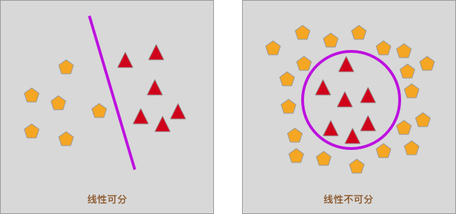
Do you still remember the above picture? When the data points are linearly separable, we can use a straight line to separate them, and the function of the dividing line is:
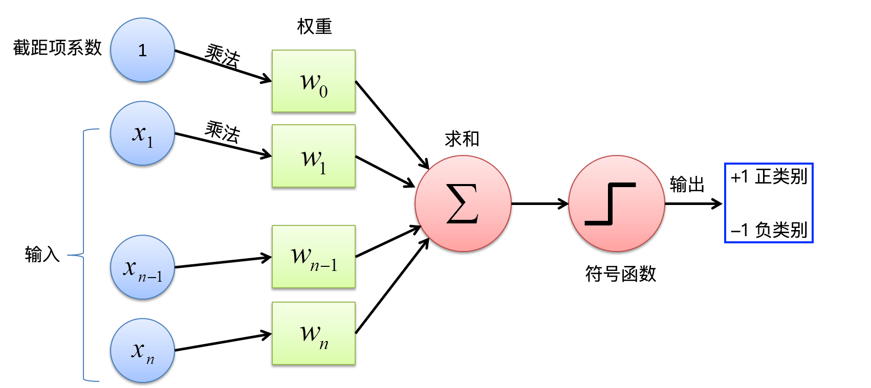
For equation (1), we can consider that the equation of the dividing line is actually obtained by multiplying each feature \(x_{1}, x_{2}, \cdots, x_{n}\) of the data set by the weights \(w_{1}, w_{2}, \cdots, w_{n}\) in turn.
After we determine the parameters of equation (1), we can obtain the corresponding function value \(f(x)\) every time we input the features \(x_{1}, x_{2}, \cdots, x_{n}\) corresponding to a data point. Then, how can we determine which class this data point belongs to?
In binary classification problems, we ultimately have two
classes, commonly referred to as the positive class and the
negative class. When we use the corresponding equation (1)
in linear regression to complete the classification,
different from passing
\(f(x)\)
into the
sigmoid
function in logistic regression, here we pass
\(f(x)\)
into the Sign function as shown below.
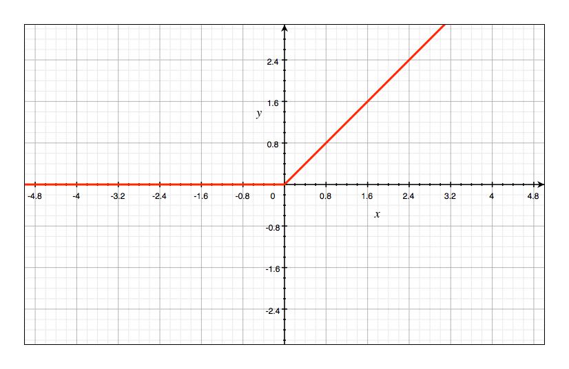
The Sign function, also known as the signum function, has only two function values. That is, when the independent variable \(x \geq 0\), the dependent variable is 1. Similarly, when \(x < 0\), the dependent variable is -1. The function graph is as follows:

Thus, when we pass \(f(x)\) in Equation (1) into Equation (2) above, we can obtain the value of \(\text{sign}(f(x))\). Among them, when \(\text{sign}(f(x)) = 1\), it is a positive classification point, and when \(\text{sign}(f(x)) = -1\), it is a negative classification point.
To sum up, we assume that the input space (feature vector) is \(X \subseteq R^n\), and the output space is \(Y = \{ -1, +1 \}\). The input \(x \subseteq X\) represents the feature vector of the instance, corresponding to the point in the input space; the output \(y \subseteq Y\) represents the category of the example. The function from the input space to the output space is as follows:
Equation (3) is called a perceptron. Note that \(f(x)\) in Equation (3) is not the same \(f(x)\) as that in Equation (1).
48.5. Perceptron Calculation Flowchart#
Above, we conducted a mathematical derivation for the perceptron. To more clearly show the calculation process of the perceptron, we have drawn the following flowchart.
48.6. Loss Function of the Perceptron#
In the previous experiments, we have introduced the definition of the loss function. During the learning process of the perceptron, we also need to determine the parameters corresponding to each feature variable, and the minimum value of the loss function often means the best parameters. So, what is the learning strategy of the perceptron, that is, what form of loss function does it usually adopt?
As shown in the following figure, when we use a straight line to separate a linearly separable data set, there may be a situation of “misclassification”.
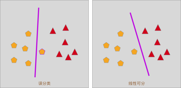
During the learning process of the perceptron, we usually use the distance from the misclassified points to the separating line (plane) to define the loss function.
48.6.1. Distance from a Point to a Line#
In middle school, we learned the derivation of the distance formula from a point to a line. For any point \(x_0\) in the \(n\)-dimensional real vector space, the distance to the line \(W*x + b = 0\) is:
Among them, \(||W||\) represents the \(L_2\) norm, that is, taking the square root of the sum of the squares of each element of the vector.
For the point \((x_i, y_i)\), when using formula \((3)\) for classification, if \(W*x_i + b > 0\), then \(sign(W*x_i + b) = 1\). In this case, the predicted classification of this point is \(+1\), and conversely, the predicted classification is \(-1\).
If the true classification of this point is different from the predicted classification, it is called a misclassified point. For a misclassified point, the true \(y_i = +1\), but \(W * x_i + b < 0\) calculated by the perceptron; or the true \(y_i = -1\), but \(W * x_i + b > 0\) calculated by the perceptron. In both cases, \(y_i(W * x_{i}+ b) < 0\) holds, that is, for misclassified points, formula \((5)\) holds.
Substitute the coordinates \((x_i, y_i)\) of the misclassified point into formula \((4)\). By comparing the magnitude of \(W * x_i + b\) with \(0\) to remove the absolute value, the distance from the misclassified point to the dividing line (plane) can be obtained as:
Thus, assuming that the set of all misclassified points is \(M\), the distance from all misclassified points to the dividing line (plane) is:
Finally, the loss function of the perceptron is obtained as:
It can be seen from formula (8) that the loss function \(J(W, b)\) is non - negative. That is to say, when there are no misclassified points, the value of the loss function is 0. At the same time, the fewer the misclassified points are, the closer the misclassified points are to the dividing line (plane), and the smaller the value of the loss function is. Meanwhile, the loss function \(J(W, b)\) is a continuously differentiable function.
48.7. Stochastic Gradient Descent Method#
When we are implementing classification, the ultimate result we want is definitely to have no misclassified points, that is, the result when the loss function takes the minimum value. In the experiment of logistic regression, in order to find the minimum value of the loss function, we use a method called Gradient Descent. And in today’s experiment, we will try an improved method of gradient descent, which is also called Stochastic Gradient Descent (abbreviation: SGD).
When using SGD to calculate the minimum value of formula (8), first arbitrarily select a dividing plane \(W_0\) and \(b_0\), and then continuously minimize the loss function using the gradient descent method:
The characteristic of stochastic gradient descent is that during the minimization process, instead of performing gradient descent on all misclassified points in \(M\) at once, it randomly selects one misclassified point each time to perform gradient descent. After updating \(W\) and \(b\), another misclassified point is randomly selected the next time to perform gradient descent until convergence.
Calculate the partial derivatives of the loss function:
If \(y_i(W * x_{i}+b)\leq0\), update \(W\) and \(b\):
Similar to the previous gradient descent, \(\lambda\) is the learning rate, which is the step size for each gradient descent. Next, we use Python to implement the above stochastic gradient descent algorithm.
from sklearn.utils import shuffle


def perceptron_sgd(X, Y, alpha, epochs):
    """
    参数:
    X -- 自变量数据矩阵
    Y -- 因变量数据矩阵
    alpha -- lamda 参数
    epochs -- 迭代次数

    返回:
    w -- 权重系数
    b -- 截距项
    """
    # 感知机随机梯度下降算法实现
    w = np.zeros(len(X[0]))  # 初始化参数为 0
    b = np.zeros(1)

    for t in range(epochs):  # 迭代
        # 每一次迭代循环打乱训练样本
        # X, Y = shuffle(X, Y)
        for i, x in enumerate(X):
            if ((np.dot(X[i], w) + b) * Y[i]) <= 0:  # 判断条件
                w = w + alpha * X[i] * Y[i]  # 更新参数
                b = b + alpha * Y[i]

    return w, b
Note
Theoretically, during the calculation of stochastic gradient descent, the sample data needs to be randomly shuffled for each iteration update. However, for the convenience of controlling the uniqueness of the subsequent content output and facilitating the explanation of the course content, the relevant code is commented out in the above implementation. You can uncomment and re-run it after finishing the course content.
The stochastic gradient descent method is a great invention. Since the datasets faced by deep learning in solving problems are very large, the traditional gradient descent has low computational efficiency on the entire dataset. However, SGD only calculates one sample at a time, so its computational speed is very fast and it is suitable for online model updates.
Of course, since SGD updates based on a single sample, it is also very easy to cause fluctuations in the loss and may not be able to reach the optimal point. For example, the following is a schematic diagram showing the剧烈波动 of the objective function optimized by SGD. (这里“剧烈波动”直接保留中文更合适,因为英文中没有完全对应的简洁表达能准确传达这个意思,如果强行翻译可能会使表达变得复杂且不准确)
However, this kind of oscillatory fluctuation also has certain advantages. Among them, compared with the fact that the gradient descent method converges on non-convex functions and may cause the loss function to fall into a local minimum, the oscillatory fluctuation of SGD may enable it to jump to new and potentially better local optima. Therefore, in practical applications, stochastic gradient descent is more commonly used.
In addition to the gradient descent method and the stochastic gradient descent method, there is also mini-batch gradient descent. The mini-batch gradient descent method uses a small batch of training samples for each update, which can be regarded as a compromise between gradient descent and stochastic gradient descent. We will not elaborate on it here.
48.8. Perceptron Classification Example#
In the previous content, we discussed the computational process of the perceptron, the loss function of the perceptron, and how to use stochastic gradient descent to solve the parameters of the perceptron. Having talked about so much theory, let’s look at a practical example below.
48.8.1. Example Dataset#
To facilitate plotting on a two-dimensional plane, only
data containing two feature variables is used here. The
name of the dataset is
course-12-data.csv. First, load the example data.
wget -nc https://cdn.aibydoing.com/aibydoing/files/course-12-data.csv
import pandas as pd

df = pd.read_csv("course-12-data.csv", header=0)  # 加载数据集
df.head()  # 预览前 5 行数据
| X0 | X1 | Y | |
|---|---|---|---|
| 0 | 5.1 | 3.5 | -1 |
| 1 | 4.9 | 3.0 | -1 |
| 2 | 4.7 | 3.2 | -1 |
| 3 | 4.6 | 3.1 | -1 |
| 4 | 5.0 | 3.6 | -1 |
It can be seen that this dataset has two feature
variables,
X0
and
X1, and a target value
Y. Among them, the target value
Y
only contains
-1
and
1. We try to plot this dataset to see the distribution of
the data.
from matplotlib import pyplot as plt

%matplotlib inline

# 绘制数据集
plt.figure(figsize=(10, 6))
plt.scatter(df["X0"], df["X1"], c=df["Y"])
<matplotlib.collections.PathCollection at 0x155a2e9e0>

48.8.2. Perceptron Training#
Next, we will use the perceptron to find the optimal separation line.
import numpy as np

X = df[["X0", "X1"]].values
Y = df["Y"].values

alpha = 0.1
epochs = 150

perceptron_sgd(X, Y, alpha, epochs)
(array([ 4.93, -6.98]), array([-3.3]))
Thus, the equation of the optimal separation line we obtained is:
At this time, the classification accuracy can be calculated:
L = perceptron_sgd(X, Y, alpha, epochs)
w1 = L[0][0]
w2 = L[0][1]
b = L[1]

z = np.dot(X, np.array([w1, w2]).T) + b
np.sign(z)
array([-1., -1., -1., -1., -1., -1., -1., -1., -1., -1., -1., -1., -1.,
       -1., -1., -1., -1., -1., -1., -1., -1., -1., -1., -1., -1.,  1.,
       -1., -1., -1., -1., -1., -1., -1., -1., -1., -1., -1., -1., -1.,
       -1., -1.,  1., -1., -1., -1., -1., -1., -1., -1., -1.,  1.,  1.,
        1.,  1.,  1.,  1.,  1.,  1.,  1.,  1.,  1.,  1.,  1.,  1.,  1.,
        1.,  1.,  1.,  1.,  1.,  1.,  1.,  1.,  1.,  1.,  1.,  1.,  1.,
        1.,  1.,  1.,  1.,  1.,  1.,  1.,  1.,  1.,  1.,  1.,  1.,  1.,
        1.,  1.,  1.,  1.,  1.,  1.,  1.,  1.,  1.,  1.,  1.,  1.,  1.,
        1.,  1.,  1.,  1.,  1.,  1.,  1.,  1.,  1.,  1.,  1.,  1.,  1.,
        1.,  1.,  1.,  1.,  1.,  1.,  1.,  1.,  1.,  1.,  1.,  1.,  1.,
        1.,  1.,  1.,  1.,  1.,  1.,  1.,  1.,  1.,  1.,  1.,  1.,  1.,
        1.,  1.,  1.,  1.,  1.,  1.,  1.])
For convenience, we directly use the accuracy calculation
method
accuracy_score()
provided by scikit-learn. You must be very familiar with
this method.
from sklearn.metrics import accuracy_score

accuracy_score(Y, np.sign(z))
0.9866666666666667
Therefore, the final classification accuracy is
approximately
0.987.
48.8.3. Plot the decision boundary line#
# 绘制轮廓线图,不需要掌握
plt.figure(figsize=(10, 6))
plt.scatter(df["X0"], df["X1"], c=df["Y"])

x1_min, x1_max = (
    df["X0"].min(),
    df["X0"].max(),
)
x2_min, x2_max = (
    df["X1"].min(),
    df["X1"].max(),
)

xx1, xx2 = np.meshgrid(np.linspace(x1_min, x1_max), np.linspace(x2_min, x2_max))
grid = np.c_[xx1.ravel(), xx2.ravel()]

probs = (np.dot(grid, np.array([L[0][0], L[0][1]]).T) + L[1]).reshape(xx1.shape)
plt.contour(xx1, xx2, probs, [0], linewidths=1, colors="red")
<matplotlib.contour.QuadContourSet at 0x154488d00>

As can be seen, the red straight line in the above figure is our final dividing line, and the classification effect is quite good.
48.8.4. Plot the transformation curve of the loss function#
In addition to plotting the decision boundary, that is, the dividing line. We can also plot the change process of the loss function to see the execution process of gradient descent.
def perceptron_loss(X, Y, alpha, epochs):
    """
    参数:
    X -- 自变量数据矩阵
    Y -- 因变量数据矩阵
    alpha -- lamda 参数
    epochs -- 迭代次数

    返回:
    loss_list -- 每次迭代损失函数值列表
    """
    # 计算每次迭代后的损失函数值
    w = np.zeros(len(X[0]))  # 初始化参数为 0
    b = np.zeros(1)
    loss_list = []

    for t in range(epochs):  # 迭代
        loss_init = 0
        for i, x in enumerate(X):
            # 每一次迭代循环打乱训练样本
            # X, Y = shuffle(X, Y)
            if ((np.dot(X[i], w) + b) * Y[i]) <= 0:  # 判断条件
                loss_init += (np.dot(X[i], w) + b) * Y[i]
                w = w + alpha * X[i] * Y[i]  # 更新参数
                b = b + alpha * Y[i]
        loss_list.append(loss_init * -1)

    return loss_list
loss_list = perceptron_loss(X, Y, alpha, epochs)

plt.figure(figsize=(10, 6))
plt.plot([i for i in range(len(loss_list))], loss_list)
plt.xlabel("Learning rate {}, Epochs {}".format(alpha, epochs))
plt.ylabel("Loss function")
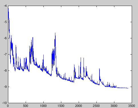
Text(0, 0.5, 'Loss function')

As shown in the figure above, you will find that after we iterate 150 times with a learning rate of 0.1, the loss function still cannot reach 0. Generally, when our data is not linearly separable, the loss function will show the oscillating linearity as shown in the figure above. Of course, this actually also reflects the oscillating fluctuations in the change of the objective function curve when applying SDG as described above.
However, if you carefully observe the scatter plot of the data above, you will find that this dataset seems to be linearly separable. Then, when the dataset is linearly separable but the transformation curve of the loss function oscillates, there are generally two reasons: the learning rate is too large or the number of iterations is too small.
Among them, it is easy to understand that the number of iterations is too small, that is to say, the number of iterations we have carried out is not enough to find the minimum value. As for whether the learning rate is too small or too large, you can refer to the following schematic diagram.

As shown in the figure above, when our learning rate is too large, it is often easy to oscillate back and forth at the bottom of the loss function and unable to reach the minimum point. Therefore, in the face of the above situation, we can adopt the method of reducing the learning rate and increasing the number of iterations to find the minimum point of the loss function.
So, let’s try again below.
alpha = 0.05  # 减小学习率
epochs = 1000  # 增加迭代次数

loss_list = perceptron_loss(X, Y, alpha, epochs)

# Flatten the arrays in loss_list
flattened_loss = [
    item[0] if isinstance(item, np.ndarray) else item for item in loss_list
]

plt.figure(figsize=(10, 6))
plt.plot(range(len(flattened_loss)), flattened_loss)
plt.xlabel("Iterations")
plt.ylabel("Loss function")
Text(0, 0.5, 'Loss function')

It can be seen that when the number of iterations is about 700 times, that is, the latter half of the above figure, the value of the loss function is equal to 0. According to what we introduced in the previous section, when the loss function is 0, it means that there are no misclassified points.
At this time, we calculate the classification accuracy again.
L = perceptron_sgd(X, Y, alpha, epochs)
z = np.dot(X, L[0].T) + L[1]
accuracy_score(Y, np.sign(z))
1.0
Consistent with the conclusion drawn from the loss function change curve, the classification accuracy rate has reached 100%, indicating that all data points are correctly classified.
48.9. Artificial Neural Network#
In the above content, we have learned what a perceptron is and how to build a perceptron classification model. You will find that a perceptron can only handle binary classification problems and must be linearly separable problems. If so, the limitations of this method are relatively large. Then, when faced with linearly inseparable or multi-classification problems, do we have a better method?
48.10. Multilayer Perceptron and Artificial Neural Network#
Here, we come to the protagonist of this article, that is, the Artificial Neural Network (ANN for short). If you come into contact with the artificial neural network for the first time, don’t think of it as too mysterious. In fact, the above perceptron model is an artificial neural network, but it is a simple single-layer neural network. And if we want to solve linearly inseparable or multi-classification problems, we often try to combine multiple perceptrons together to form a more complex neural network structure.
{note}
Due to some historical issues, the boundaries between the three terms perceptron, multilayer perceptron, and artificial neural network are blurred. In this experiment, the artificial neural network introduced here refers to the multilayer perceptron in a sense.
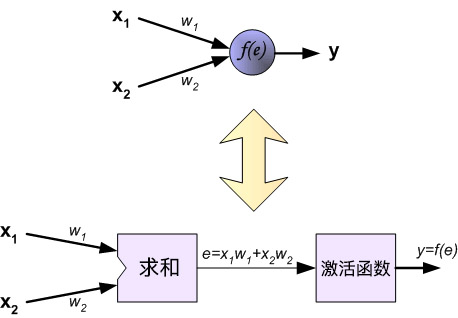
In the above text, we showed the working process of the perceptron through a diagram, and we further streamlined this flowchart as follows:
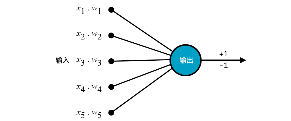
This diagram shows the execution process of a perceptron model. We can call the input the “input layer” and the output the “output layer”. A network structure like this that only contains an input layer can be called a single-layer neural network structure.
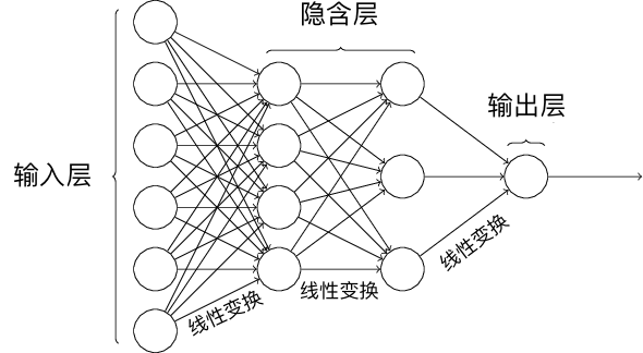
A single perceptron forms a single-layer neural network. If we use the output of one perceptron as the input of another perceptron, we form a multilayer perceptron, which is a multi-layer neural network. Among them, the layers between the input and output layers are called hidden layers. As shown in the following figure, this is the neural network structure with 1 hidden layer.
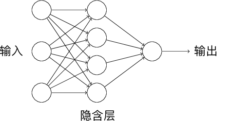
When calculating the number of layers in a neural network structure, we generally only count the number of input and hidden layers. That is, the above is a two-layer neural network structure.
48.11. Activation Function#
At present, we have come into contact with four concepts: logistic regression, perceptron, multilayer perceptron, and artificial neural network. You may vaguely feel that these four methods seem to be related to linear functions, and the difference lies in the different ways of dealing with the dependent variable of the linear function.
-
For logistic regression, we use the sigmoid function to convert \(f(x)\) into a probability, ultimately achieving binary classification.
-
For the perceptron, we use the sign function to convert \(f(x)\) into -1 and +1, ultimately achieving binary classification.
-
For the multilayer perceptron, which has a multi-layer neural network structure, there are generally more operations in the way of dealing with \(f(x)\).
Thus, the sigmoid function and the sign function have another name, called the “Activation function”. When you hear about the activation function, don’t think it’s something extremely advanced at first. The reason for this name is that the function itself has some characteristics, but ultimately it is still a mathematical function. Next, we will list some common activation functions and their graphs.
48.11.1. sigmoid function#
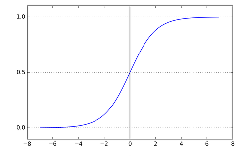
The sigmoid function should be quite familiar, and its formula is as follows:
The graph of the sigmoid function is S-shaped, and the function values are between (0, 1):
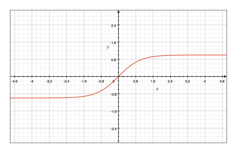
48.11.2. Tanh Function#
The graph of the Tanh function is very similar to that of the sigmoid function, both being S-shaped. However, the values of the Tanh function are between (-1, 1), and the formula is as follows:
48.11.3. ReLU Function#
The full name of the ReLU function is Rectified Linear Unit, that is, the rectified linear unit. The formula is as follows:
The ReLU has many advantages. For example, the convergence speed is relatively fast and it is not easy to have the vanishing gradient problem. Since this will not be used in this experiment, we will talk about it later. The graph of ReLU is as follows:
48.11.4. The Role of Activation Functions#
The above lists 3 commonly used activation functions, among which the sigmoid function is a very commonly used activation function in the artificial neural network introduced today. Speaking straightforwardly about the role of activation functions, it is to perform non-linear transformations on data. It’s just that different activation functions are suitable for different scenarios, and these are all summarized by machine learning experts based on application experience.
In the neural network structure, we continuously connect the input and output through linear functions. You can imagine that in this structure, the output of each layer is a linear transformation of the input of the upper layer. Thus, no matter how many layers the neural network has, the final output is a linear combination of the input. In this case, what’s the difference between a single-layer neural network and a multi-layer neural network? (There is no difference)
As shown in the figure above, multiple combinations of linear transformations are still linear transformations. If we add activation functions to the network structure, it is equivalent to introducing non-linear factors, which can solve classification tasks that cannot be completed by linear models.
48.12. Intuitive Understanding of Backpropagation Algorithm (BP)#
In the previous section on perceptrons, we defined a loss function and used a method called stochastic gradient descent to find the optimal parameters. If you observe the process of stochastic gradient descent carefully, it is actually about solving partial derivatives and combining them into gradients to update the weights \(W\) and \(b\). Since the perceptron has only a single-layer network structure, the process of solving the gradient is relatively simple. However, when we combine multiple layers of neural networks, the process of updating the weights becomes more complex, and the backpropagation algorithm was born precisely to quickly solve for the gradient.
The backpropagation algorithm is simple to describe but rather complex to understand smoothly. Here, we have cited an illustration from a popular science article to assist in understanding the backpropagation process.
The following figure presents a classic three-layer neural network structure, which includes two inputs \(x_{1}\) and \(x_{2}\) and one output \(y\).
Each purple unit in the network represents an independent neuron, which is composed of two units respectively. One unit is the weight and the input signal, while the other is the activation function mentioned above. Among them, \(e\) represents the activation signal, so \(y = f(e)\) is the non-linear output after being processed by the activation function, that is, the output of the entire neuron.
Next, start training the neural network. The training data consists of the input signals \(x_{1}\) and \(x_{2}\) and the expected output \(z\). First, calculate the value corresponding to the first neuron \(y_{1} = f_{1}(e)\) in the first hidden layer.
Next, calculate the value corresponding to the second neuron \(y_{2} = f_{2}(e)\) in the first hidden layer.
Then, calculate the value corresponding to the third neuron \(y_{3} = f_{3}(e)\) in the first hidden layer.
Similar to the process of calculating the first hidden layer, we can calculate the values of the second hidden layer.
Finally, obtain the result of the output layer:
The above process is called the forward propagation process. So, what is backpropagation? Let’s continue to look:
When we obtain the output result \(y\), we can compare it with the expected output \(z\) to get the error \(\delta\).
Then, we reverse - propagate the calculated error \(\delta\) along the neuron circuit back to the previous hidden layer, and the error corresponding to each neuron is the propagated error multiplied by the weight.
Similarly, we continue to reverse - propagate the error of the second hidden layer back to the first hidden layer.
At this point, we can update the weights \(w\) between the input layer and the first hidden layer using the error propagated backward, as shown in the following figure:
Similarly, update the weights \(w\) between the first hidden layer and the second hidden layer, as shown in the following figure:
Finally, update the weights \(w\) between the second hidden layer and the output layer, as shown in the following figure:
\(\eta\) in the figure represents the learning rate. This completes one iteration process. After updating the weights, the next round of forward propagation starts to obtain the output, and then the error is backpropagated to update the weights, and this iteration continues in turn.
Therefore, backpropagation actually represents the backpropagation of error.
48.13. Python Implementation of Artificial Neural Network#
In the above content, we introduced the composition of the artificial neural network and the most important backpropagation algorithm. Next, we will try to implement a complete process of a neural network running through Python.
48.13.1. Define the Neural Network Structure#
To make the derivation process clear enough, here we only construct an artificial neural network structure with 1 hidden layer. Among them, the input layer has 2 neurons, the hidden layer has 3 neurons, and the output layer is used to solve the 2-classification problem. The structure of this neural network is as follows:
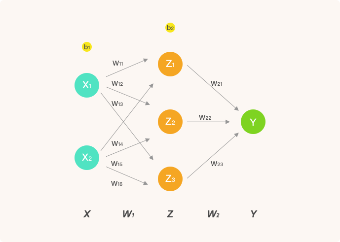
In this experiment, the activation function we used is the sigmoid function:
Since the derivative of the sigmoid function will be used below, its derivative formula is also written out:
Then, we implement formula (17) in Python:
def sigmoid(x):
    # sigmoid 函数
    return 1 / (1 + np.exp(-x))


def sigmoid_derivative(x):
    # sigmoid 函数求导
    return sigmoid(x) * (1 - sigmoid(x))
48.13.2. Forward Propagation#
In forward propagation, the computational process for each neuron is: linear transformation → activation function → output value.
Meanwhile, we make the following convention:
-
\(Z\) represents the output of the hidden layer, and \(Y\) is the final output of the output layer.
-
\(w_{ij}\) represents the \(j\)-th weight from the \(i\)-th layer.
Thus, the algebraic calculation process of the forward propagation in the above figure is as follows.
The input of the neural network is \(X\), the weights of the first layer are \(W_1\), and the weights of the second layer are \(W_2\). For the convenience of demonstration, \(X\) is a single sample. Since it is matrix operation, it is very easy for us to expand it to multi-sample input.
Next, calculate the output \(Z\) of the hidden layer neurons (linear transformation → activation function). Similarly, for the sake of clarity in the calculation process, we represent the intercept term as 0 here.
Finally, calculate the output layer \(Y\) (linear transformation → activation function):
Next, implement the forward propagation calculation process and convert the above formula into code as follows:
# 示例样本
X = np.array([[1, 1]])
y = np.array([[1]])

X, y
(array([[1, 1]]), array([[1]]))
Then, randomly initialize the weights of the hidden layer.
W1 = np.random.rand(2, 3)
W2 = np.random.rand(3, 1)

W1, W2
(array([[0.28554135, 0.43250251, 0.7229516 ],
        [0.50588839, 0.14166136, 0.85064831]]),
 array([[0.3809778 ],
        [0.8640332 ],
        [0.17770754]]))
The forward propagation process is implemented based on equations (21) and (22).
input_layer = X  # 输入层
hidden_layer = sigmoid(np.dot(input_layer, W1))  # 隐含层,公式 20
output_layer = sigmoid(np.dot(hidden_layer, W2))  # 输出层,公式 22

output_layer
array([[0.72354249]])
48.13.3. Backpropagation#
Next, we use the gradient descent method to optimize the parameters of the neural network. First, we need to define the loss function, and then calculate the partial derivatives (gradients) of the loss function with respect to the weights of each layer in the neural network.
At this time, let the output value of the neural network be \(Y\) and the true value be \(y\). Then, define the squared loss function as follows:
Next, to solve the gradient \(\frac{\partial Loss(y, Y)}{\partial{W_2}}\), the chain rule of differentiation needs to be used:
Similarly, the gradient \(\frac{\partial Loss(y, Y)}{\partial{W_1}}\) is obtained as follows:
Among them, \(\frac{\partial Y}{\partial{W_2}}\) and \(\frac{\partial Y}{\partial{W_1}}\) are obtained through formulas (22) and (21) respectively. Next, we implement the code for the backpropagation process based on the formulas.
# 公式 24
d_W2 = np.dot(
    hidden_layer.T,
    (2 * (output_layer - y) * sigmoid_derivative(np.dot(hidden_layer, W2))),
)

# 公式 25
d_W1 = np.dot(
    input_layer.T,
    (
        np.dot(
            2 * (output_layer - y) * sigmoid_derivative(np.dot(hidden_layer, W2)), W2.T
        )
        * sigmoid_derivative(np.dot(input_layer, W1))
    ),
)

d_W2, d_W1
(array([[-0.07610733],
        [-0.07075271],
        [-0.09160865]]),
 array([[-0.0090425 , -0.02202468, -0.00279526],
        [-0.0090425 , -0.02202468, -0.00279526]]))
Now, the learning rate can be set, and \(W_1\) and \(W_2\) can be updated once.
# 梯度下降更新权重, 学习率为 0.05

W1 -= 0.05 * d_W1  # 如果上面是 y - output_layer,则改成 +=
W2 -= 0.05 * d_W2

W2, W1
(array([[0.38478317],
        [0.86757083],
        [0.18228797]]),
 array([[0.28599347, 0.43360375, 0.72309136],
        [0.50634052, 0.1427626 , 0.85078807]]))
Above, we have implemented 1 forward → backward pass of a single sample in the neural network and completed 1 weight update using gradient descent. Then, below we will fully implement this network and learn from a multi-sample dataset.
# 示例神经网络完整实现
class NeuralNetwork:
    # 初始化参数
    def __init__(self, X, y, lr):
        self.input_layer = X
        self.W1 = np.random.rand(self.input_layer.shape[1], 3)
        self.W2 = np.random.rand(3, 1)
        self.y = y
        self.lr = lr
        self.output_layer = np.zeros(self.y.shape)

    # 前向传播
    def forward(self):
        self.hidden_layer = sigmoid(np.dot(self.input_layer, self.W1))
        self.output_layer = sigmoid(np.dot(self.hidden_layer, self.W2))

    # 反向传播
    def backward(self):
        d_W2 = np.dot(
            self.hidden_layer.T,
            (
                2
                * (self.output_layer - self.y)
                * sigmoid_derivative(np.dot(self.hidden_layer, self.W2))
            ),
        )

        d_W1 = np.dot(
            self.input_layer.T,
            (
                np.dot(
                    2
                    * (self.output_layer - self.y)
                    * sigmoid_derivative(np.dot(self.hidden_layer, self.W2)),
                    self.W2.T,
                )
                * sigmoid_derivative(np.dot(self.input_layer, self.W1))
            ),
        )

        # 参数更新
        self.W1 -= self.lr * d_W1
        self.W2 -= self.lr * d_W2
Next, we use the example dataset at the beginning of the experiment for testing. First, we need to adjust the data shape to meet the requirements.
X = df[["X0", "X1"]].values  # 输入值
y = df[["Y"]].values  # 真实 y
Next, we input it into the network and iterate 100 times:
nn = NeuralNetwork(X, y, lr=0.001)  # 定义模型
loss_list = []  # 存放损失数值变化

for i in range(100):
    nn.forward()  # 前向传播
    nn.backward()  # 反向传播
    loss = np.sum((y - nn.output_layer) ** 2)  # 计算平方损失
    loss_list.append(loss)

print("final loss:", loss)
plt.plot(loss_list)  # 绘制 loss 曲线变化图
final loss: 133.26148346146633
[<matplotlib.lines.Line2D at 0x156b4e470>]

It can be seen that the loss function gradually decreases and approaches convergence, and the change curve is much smoother than that calculated by the perceptron. However, since we removed the intercept term and the network structure is too simple, the convergence situation is not ideal. The focus of this experiment is to understand the intermediate process of BP, and it is impossible to have both high accuracy and low learning difficulty. In addition, it should be noted that since the weights are randomly initialized, the results of multiple runs will be different.
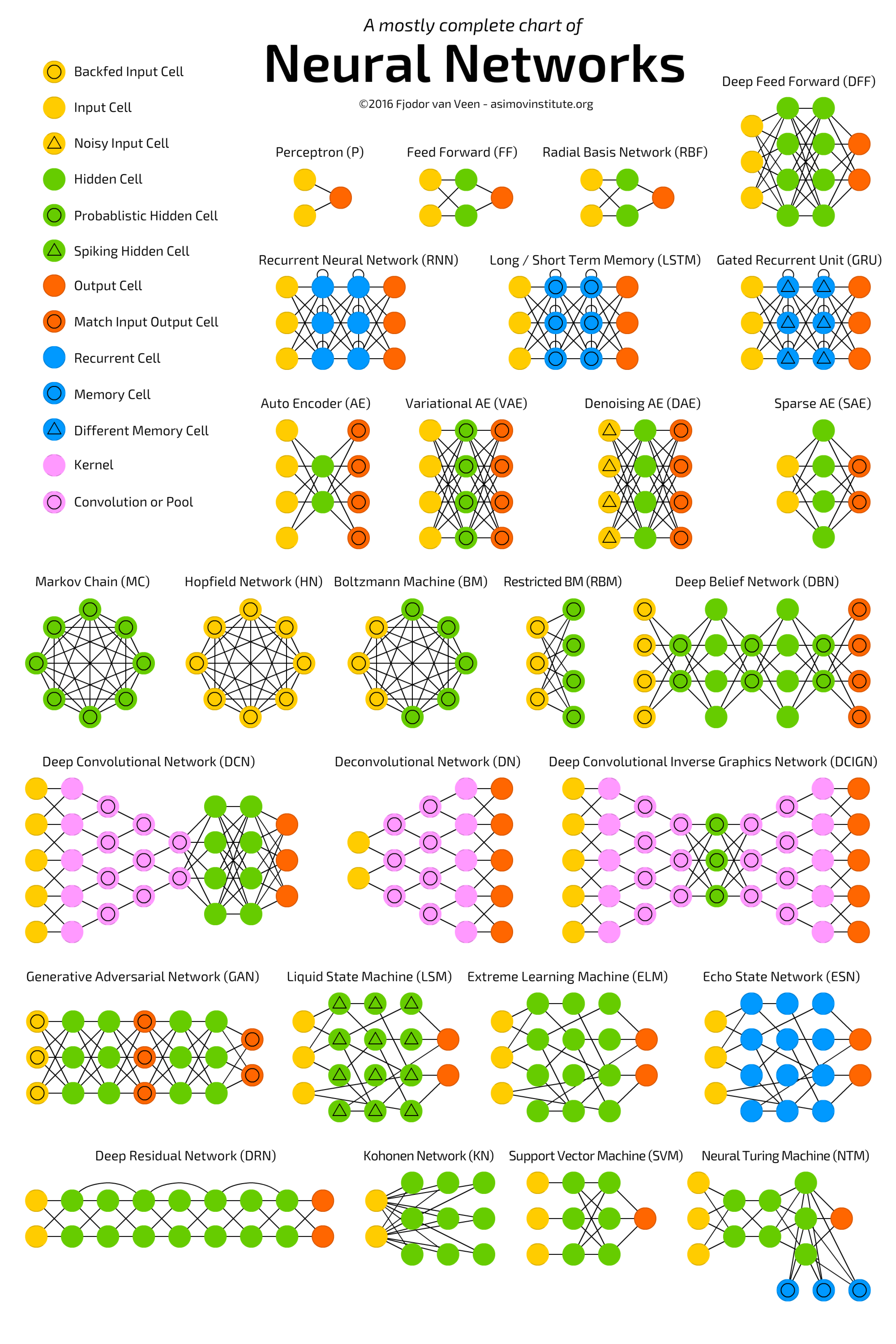
So far, we have completed the training of a simple artificial neural network. In fact, this is just the tip of the iceberg of artificial neural networks, and this basic and simple neural network structure is often used in the process of solving real problems. Later, we will learn more complex neural network structures. The article THE NEURAL NETWORK ZOO has sorted out a large number of different types of neural networks. I believe you can feel the wonderful world of artificial neural networks from the following figure.
48.14. Supplementary Videos#
Deep learning is actually the application of artificial neural networks. The well-known foreign popular science video author 3Blue1Brown has produced 4 videos explaining artificial neural networks, which we supplement below for your reference. Since the copyright owner of the videos, 3Blue1Brown, does not allow reprinting, you need to jump to the following link to watch.
48.15. Summary#
Starting from the principle of the perceptron, this experiment guided everyone to build a single-layer neural network structure in Python and completed data classification. Subsequently, the experiment introduced the concept of multi-layer artificial neural networks through the perceptron, and learned about the widely used backpropagation algorithm in neural network calculations through accompanying diagrams. Finally, a complete two-layer neural network structure was built in Python. After mastering these contents, the learning requirements of artificial neural networks have been met.
Related Links