58. PyTorch Implementation of Linear Regression#
58.1. Introduction#
The previous experiments have provided a detailed introduction to the use of PyTorch. I believe you are already familiar with PyTorch’s tensor types, common operation methods, and the process of building neural networks. In this challenge, you are required to use PyTorch to implement the well-known linear regression. Although linear regression is simple, the purpose of the challenge is to get familiar with the use of PyTorch.
58.2. Key Points#
Principles and Usage of PyTorch
-
Implementing Linear Regression with the nn.Module Class
Linear regression is already an old acquaintance of ours, and it was introduced in depth at the beginning of the course. If we were to summarize linear regression in one sentence, it would be to model the relationship between input and output data using a linear method.
First, we generate the sample data required for this challenge. Here, we use the APIs provided by PyTorch to operate.
import torch
from matplotlib import pyplot as plt

%matplotlib inline

torch.manual_seed(10)  # 随机数种子
x = torch.linspace(1, 10, 50)  # 生成等间距张量
y = 2 * x + 3 * torch.rand(50)

plt.style.use("ggplot")  # 使用 ggplot 绘图样式
plt.scatter(x, y)
<matplotlib.collections.PathCollection at 0x12ea2de40>

58.3. Implementing the Linear Regression Model#
As mentioned in the previous experimental content, the
torch.nn.Module
class is the base class for all neural networks. It can
represent either a single layer in a neural network or a
neural network consisting of multiple layers. Next, you will
implement the
LinearRegressionModel()
linear regression class required for the challenge by
inheriting from the
torch.nn.Modules
class.
Exercise 58.1
Challenge: Implement the
LinearRegressionModel()
linear regression class required for the challenge by
inheriting from the
torch.nn.Module
class.
Requirement: Only use the classes and methods provided by PyTorch.
Hint: You may use the
nn.Linear()
linear transformation layer.
import torch.nn as nn

## 代码开始 ### (> 5 行代码)

## 代码结束 ###
Solution to Exercise 58.1
import torch.nn as nn

### Code start ### (> 5 lines of code)
class LinearRegressionModel(nn.Module):
    def __init__(self):
        super(LinearRegressionModel, self).__init__()
        self.linear = nn.Linear(1, 1)

    def forward(self, x):
        out = self.linear(x)
        return out
### Code end ###
Run the tests
LinearRegressionModel()
Expected output
LinearRegressionModel(
  (linear): Linear(in_features=1, out_features=1, bias=True)
)
In this challenge, the least squares method will not be used to solve the linear regression parameters. Instead, an iterative method will be used. Therefore, first, the loss function and the optimizer need to be defined. The challenge will choose the value of MSE as the loss function and solve it through the SGD algorithm.
Exercise 58.2
Challenge: Define the MSE loss function and the Stochastic Gradient Descent optimizer.
Requirement: Set the learning rate of the Stochastic Gradient Descent optimizer to 0.01, and use the default parameters for the rest.
Hint: You may use the loss function and optimizer mentioned in the experiment.
model = LinearRegressionModel()  # 实例化模型

## 代码开始 ### (≈ 2 行代码)
loss_fn = None
opt = None
## 代码开始 ### (≈ 3 行代码)
Solution to Exercise 58.2
model = LinearRegressionModel()  # Instantiate the model

### Start of code ### (≈ 2 lines of code)
loss_fn = nn.MSELoss()  # Define the loss function
opt = torch.optim.SGD(model.parameters(), lr=0.01)  # Define the optimizer
### End of code ### (≈ 3 lines of code)
Run the test
loss_fn, opt
Expected output
(MSELoss(), SGD (
 Parameter Group 0
     dampening: 0
     lr: 0.01
     momentum: 0
     nesterov: False
     weight_decay: 0
 ))
Everything is ready. Next is to train the model and solve for the linear regression parameters.
Exercise 58.3
Challenge: Complete the iterative process of optimizing the linear regression parameters.
Requirement: The number of iterations is 100.
Hint: Pay attention to the shape problem of the input data. The idea is to first perform a forward pass to obtain the true values, calculate the loss, and iterate through the optimizer.
## 代码开始 ### (> 5 行代码)

## 代码结束 ###
Solution to Exercise 58.3
### Code start ### (> 5 lines of code)
iters = 100
for i in range(iters):

    x = x.reshape(len(x), 1)  # Input x tensor
    y = y.reshape(len(x), 1)  # Input y tensor

    y_ = model(x)  # Forward pass
    loss = loss_fn(y_, y)  # Calculate loss

    opt.zero_grad()  # Clear the optimizer gradient, otherwise it will accumulate
    loss.backward()  # Backward propagate from the last loss
    opt.step()  # Optimizer iteration

    if (i+1) % 10 == 0:
        print('Iteration [{}/{}], Loss: {:.3f}'
             .format(i+1, iters, loss.item()))
### Code end ###
Expected output: (It doesn’t matter if the loss values are different)
Iteration [ 10/100], Loss: 0.791
Iteration [ 20/100], Loss: 0.784
Iteration [ 30/100], Loss: 0.778
Iteration [ 40/100], Loss: 0.772
Iteration [ 50/100], Loss: 0.767
Iteration [ 60/100], Loss: 0.762
Iteration [ 70/100], Loss: 0.757
Iteration [ 80/100], Loss: 0.753
Iteration [ 90/100], Loss: 0.749
Iteration [100/100], Loss: 0.745
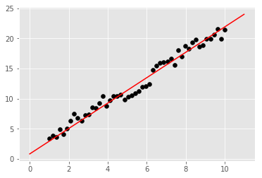
Finally, it is also necessary to plot the fitted line on the original scatter plot to check the effect.
Exercise 58.4
Challenge: Plot the fitted line onto the image according to the fitted parameters.
Hint: Read the fitted parameters via
model.state_dict().
## 代码开始 ### (≈ 4 行代码)

## 代码结束 ###
Solution to Exercise 58.4
### Code starts ### (≈ 4 lines of code)
weight = model.state_dict()['linear.weight']  # Weight
bias = model.state_dict()['linear.bias']  # Bias term

plt.scatter(x, y, c='black')
plt.plot([0, 11], [bias, weight * 11 + bias], 'r')
### Code ends ###
Expected output