
87. Implement the Sarsa Learning Algorithm to Exit the Maze#
87.1. Introduction#
In value-based reinforcement learning, we mainly implemented the Q-Learning algorithm. In fact, the biggest difference between the Sarsa algorithm and Q-Learning lies in the update of the Q-Table. In this experiment, we combined the implementation of the Q-Learning algorithm in the experiment and completed the maze challenge according to the algorithm process of Sarsa.
87.2. Key Points#
Q-Table Initialization
Q-Table Update Function
Complete Sarsa Algorithm Implementation
87.3. Q-Table Initialization#
Based on the previous experimental content, you should know that whether it is Q-Learning or Sarsa, their core is based on value iteration, so it is necessary to initialize the Q-Table first.
{exercise-start}
:label: chapter11_03_1
Challenge: Initialize the Q-Table as required.
Requirement: Construct a \(16*4\) DataFrame table (16 states, 4 actions) as the Q-Table.
Hint: The initialization method is the same as that in the Q-Learning experiment.
{exercise-end}
import numpy as np
import pandas as pd
import time
from IPython import display


def init_q_table():
    ### 代码开始 ### (≈ 2 行代码)
    actions = None
    q_table = None
    ### 代码结束 ###

    return q_table
{solution-start} chapter11_03_1
:class: dropdown
import numpy as np
import pandas as pd
import time
from IPython import display


def init_q_table():

    ### Start of code ### (≈ 2 lines of code)
    actions = np.array(['up', 'down', 'left', 'right'])
    q_table = pd.DataFrame(np.zeros((16, len(actions))),
                           columns=actions)  # Initialize the Q-Table to all 0s
    ### End of code ###

    return q_table
{solution-end}
init_q_table()
{note}
In this course, the Notebook challenge system cannot automatically judge. You need to supplement the missing code in the above cell and run it by yourself. If the output result is the same as the expected output result below, it means that this challenge has been successfully passed. After completing all the content, click "Submit for Detection" to pass. This note will not appear again in the following.
Expected output
up |
down |
left |
right |
|
|---|---|---|---|---|
0 |
0.0 |
0.0 |
0.0 |
0.0 |
1 |
0.0 |
0.0 |
0.0 |
0.0 |
2 |
0.0 |
0.0 |
0.0 |
0.0 |
3 |
0.0 |
0.0 |
0.0 |
0.0 |
4 |
0.0 |
0.0 |
0.0 |
0.0 |
5 |
0.0 |
0.0 |
0.0 |
0.0 |
6 |
0.0 |
0.0 |
0.0 |
0.0 |
7 |
0.0 |
0.0 |
0.0 |
0.0 |
8 |
0.0 |
0.0 |
0.0 |
0.0 |
9 |
0.0 |
0.0 |
0.0 |
0.0 |
10 |
0.0 |
0.0 |
0.0 |
0.0 |
11 |
0.0 |
0.0 |
0.0 |
0.0 |
12 |
0.0 |
0.0 |
0.0 |
0.0 |
13 |
0.0 |
0.0 |
0.0 |
0.0 |
14 |
0.0 |
0.0 |
0.0 |
0.0 |
15 |
0.0 |
0.0 |
0.0 |
0.0 |
A table with a border of 1, presented as a DataFrame. The table has a header row with column names ‘up’, ‘down’, ‘left’, and ‘right’, and 16 rows with each cell in the table containing the value 0.0.
87.4. Action Selection#
Next, we need to use the
\(\epsilon\)-greedy method to select actions based on the Q-Table.
Here, we implement the
act_choose
function following the experimental content.
{exercise-start}
:label: chapter11_03_2
Challenge: Use the \(\epsilon\)-greedy method to select actions based on the Q-Table.
Specification: With a probability of
\(1 - \epsilon\), or when all Q-values are 0, select an action randomly;
otherwise, select the action according to the maximum
Q-value, and denote the action as
action.
Hint: You may use if-else statements for judgment, which is the same as in the experiment.
{exercise-end}
def act_choose(state, q_table, epsilon):
    state_act = q_table.iloc[state, :]
    actions = np.array(["up", "down", "left", "right"])

    ### 代码开始 ### (≈ 4 行代码)
    if None:
        action = None
    else:
        action = None
    ### 代码结束 ###

    return action
{solution-start} chapter11_03_2
:class: dropdown
def act_choose(state, q_table, epsilon):

    state_act = q_table.iloc[state, :]
    actions = np.array(['up', 'down', 'left', 'right'])

    ### Start of code ### (≈ 4 lines of code)
    if (np.random.uniform() > epsilon or state_act.all() == 0):
        action = np.random.choice(actions)
    else:
        action = state_act.idxmax()
    ### End of code ###

    return action
{solution-end}
Run the test
seed = np.random.RandomState(25)  # 为了保证验证结果相同引入随机数种子
a = seed.rand(16, 4)
test_q_table = pd.DataFrame(a, columns=["up", "down", "left", "right"])
l = []
for s in [1, 4, 7, 12, 14]:
    l.append(act_choose(state=s, q_table=test_q_table, epsilon=1))
l
Expected output
['left', 'right', 'right', 'right', 'left']
87.5. Action Feedback#
In the action feedback, we also set the reward at the
terminal to
10
and the penalty for falling into a hole to
-10. Also, to find the shortest path as soon as possible, the
penalty for each step is
-1. You can directly use the similar code blocks in the
experiment.
def env_feedback(state, action, hole, terminal):
    reward = 0.0
    end = 0
    a, b = state
    if action == "up":
        a -= 1
        if a < 0:
            a = 0
        next_state = (a, b)
    elif action == "down":
        a += 1
        if a >= 4:
            a = 3
        next_state = (a, b)
    elif action == "left":
        b -= 1
        if b < 0:
            b = 0
        next_state = (a, b)
    elif action == "right":
        b += 1
        if b >= 4:
            b = 3
        next_state = (a, b)

    if next_state == terminal:
        reward = 10.0
        end = 2
    elif next_state == hole:
        reward = -10.0
        end = 1
    else:
        reward = -1.0

    return next_state, reward, end
87.6. Q-Table Update#
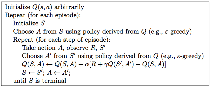
Next, it is necessary to complete the Q-Table update function. From the experimental content, it can be seen that the update of the Q-Table in Sarsa is the biggest difference from Q-Learning. Therefore, it needs to be implemented according to the Q-Table update formula of Sarsa.
{exercise-start}
:label: chapter11_03_3
Challenge: Complete the Q-Table update function according to the Q-Table update formula of Sarsa below.
Hint: Modify it in combination with the Q-Table update
function in Q-Learning. Use
.loc[]
when viewing specific values of the DataFrame by label.
{exercise-end}
def update_q_table(
    q_table, state, action, next_state, next_action, terminal, gamma, alpha, reward
):
    x, y = state
    next_x, next_y = next_state
    q_original = q_table.loc[x * 4 + y, action]

    if next_state != terminal:
        ### 代码开始 ### (≈ 1 行代码)
        q_predict = None
        ### 代码结束 ###
    else:
        q_predict = reward

    ### 代码开始 ### (≈ 1 行代码)
    q_table.loc[None] = None
    ### 代码结束 ###

    return q_table
{solution-start} chapter11_03_3
:class: dropdown
def update_q_table(q_table, state, action, next_state, next_action, terminal, gamma, alpha, reward):

    x, y = state
    next_x, next_y = next_state
    q_original = q_table.loc[x * 4 + y, action]

    if next_state!= terminal:
        ### Code starts ### (≈ 1 line of code)
        q_predict = reward + gamma * \
            q_table.loc[next_x * 4 + next_y, next_action]  # Not selected through.max()
        ### Code ends ###
    else:
        q_predict = reward

    # Code starts ### (≈ 1 line of code)
    # Consistent with Q-Learning
    q_table.loc[x * 4 + y, action] = (1-alpha) * q_original + alpha * q_predict
    ### Code ends ###

    return q_table
{solution-end}
Run the test (execute only once. Restart the kernel if you need to execute it again)
new_q_table = update_q_table(
    q_table=test_q_table,
    state=(2, 2),
    action="right",
    next_state=(2, 3),
    next_action="down",
    terminal=(3, 2),
    gamma=0.9,
    alpha=0.8,
    reward=10,
)

new_q_table.loc[10, "right"]
Expected output: (results obtained from executing only once)
8.740755431411795
Similarly, to demonstrate the effect of reinforcement learning, define a state display function. Here, you can simply reuse the corresponding code block in the experiment.
def show_state(end, state, episode, step, q_table):
    terminal = (3, 2)
    hole = (2, 1)
    env = np.array([["_ "] * 4] * 4)
    env[terminal] = "$ "
    env[hole] = "# "
    env[state] = "L "
    interaction = ""
    for i in env:
        interaction += "".join(i) + "\n"

    if state == terminal:
        message = "EPISODE: {}, STEP: {}".format(episode, step)
        interaction += message
        display.clear_output(wait=True)
        print(interaction)
        print("\n" + "q_table:")
        print(q_table)
        time.sleep(3)  # 在成功到终点时,等待 3 秒
    else:
        display.clear_output(wait=True)
        print(interaction)
        print("\n" + "q_table:")
        print(q_table)
        time.sleep(0.3)  # 在这里控制每走一步所需要时间
87.7. Sarsa Algorithm Implementation#
Finally, we implement the complete learning process according to the Sarsa algorithm pseudocode.
Exercise 87.1
Challenge: After successfully completing the above several functions, implement the complete learning process according to the following Sarsa algorithm pseudocode. Please complete the code in combination with Q-Learning.
def sarsa(max_episodes, alpha, gamma, epsilon):
    q_table = init_q_table()
    terminal = (3, 2)
    hole = (2, 1)
    episodes = 0
    while episodes < max_episodes:
        step = 0
        state = (0, 0)
        end = 0
        show_state(end, state, episodes, step, q_table)
        x, y = state

        ### 代码开始 ### (≈ 1 行代码)
        action = None  # 动作选择
        ### 代码结束 ###

        while end == 0:
            next_state, reward, end = env_feedback(
                state, action, hole, terminal
            )  # 环境反馈
            next_x, next_y = next_state
            next_action = act_choose(next_x * 4 + next_y, q_table, epsilon)  # 动作选择

            ### 代码开始 ### (≈ 3 行代码)
            q_table = None  # q-table 更新
            state = None
            action = None
            ### 代码结束 ###

            step += 1
            show_state(end, state, episodes, step, q_table)
        if end == 2:
            episodes += 1
sarsa(max_episodes=20, alpha=0.8, gamma=0.9, epsilon=0.9) # 执行测试
Expected output
_ _ _ _
_ _ _ _
_ # _ _
_ _ L _
EPISODE: 19, STEP: 5

q_table:
          up       down      left     right
0  -4.421534  -3.457078 -3.936450 -4.152483
1  -3.409185  -9.062400 -3.433181 -3.596441
2  -2.213120   4.590499 -3.514029 -3.414613
3  -1.536000  -1.574400 -2.908418 -3.936450
4  -4.109114  -2.730086 -2.836070 -2.548000
5  -2.836070  -9.984000 -2.065920 -1.720000
6  -2.850867   8.000000 -2.562662 -0.800000
7  -2.342144  -0.800000 -1.982720  0.000000
8  -2.509531  -2.348544 -2.213120 -8.000000
9   0.000000   0.000000  0.000000  0.000000
10 -3.033926  10.000000 -8.000000 -0.800000
11 -2.844488   0.000000  0.000000 -0.800000
12 -2.766862  -1.536000 -1.536000  6.142464
13  0.000000   0.000000 -2.325504  9.600000
14  0.000000   0.000000  0.000000  0.000000
15  0.000000   0.000000  0.000000  0.000000
Since the values in the Q Table are random, the above experimental results are for reference only. As long as the Q Table is continuously updated as required with the increase in the number of iterations, and the number of steps taken by the agent becomes fewer, eventually approaching 5 steps, it is fine.