73. Text Classification Principles and Practices#
73.1. Introduction#
Natural Language Processing (NLP) is a sub-discipline in the fields of artificial intelligence and linguistics, mainly focusing on exploring how to process and utilize natural language. Natural language processing encompasses multiple aspects and steps, such as cognitive, understanding, generation, etc. This experiment will focus on the application of text classification in natural language processing.
73.2. Key Points#
Text classification process
Chinese text tokenization
English text tokenization
Text feature extraction
Fake news classification task
In this experiment, we mainly focus on the methods related to text classification in natural language applications.
Text classification is a problem that people often encounter in their daily work and is also an important research area in machine learning and natural language processing. In the general sense, text classification is actually just symbolic labels (i.e., natural numbers), without additional procedural or explanatory knowledge, nor metadata (such as Chinese Library Classification numbers). Information can only be extracted from the content of the document itself to classify the document. Of course, for specific applications, using external knowledge or metadata can improve the generalization ability of the classifier.
So, for a text classification problem, we generally follow the following process to handle it:

In language understanding, words are the smallest meaningful units that can act independently. From words to sentences, and from sentences to texts. Therefore, text tokenization is generally the first step in natural language processing. After tokenizing a sentence, it is still impossible to classify it because machines cannot understand natural languages that humans can use. So, next, words need to be processed into vectors that can be input into algorithms, and different vectorization and preprocessing methods are collectively referred to as the process of feature extraction. Finally, a machine learning classification model can be established based on text features to complete text classification.
73.3. Chinese Text Tokenization#
Since the concept of Chinese word segmentation was proposed, after years of development, it can be mainly divided into three methods: mechanical word segmentation method, statistical word segmentation method, and the combination of the two.
Among them, the mechanical word segmentation method is also called the rule-based word segmentation method. This word segmentation method matches the string to be processed with the words in a word list dictionary one by one according to certain rules. If a certain string is found in the dictionary, it is segmented; otherwise, it is not segmented. According to the matching rules, the mechanical word segmentation method can be further divided into three types: forward maximum matching method, backward maximum matching method, and bidirectional matching method.
73.3.1. Forward Maximum Matching Method#
The Forward Maximum Match Method (Maximum Match Method, abbreviated as: MM) means to match with the words in the dictionary from left to right according to the maximum principle. Suppose the longest word in the dictionary is \(m\) characters. Then take \(m\) characters from the leftmost of the text to be segmented and match them with the dictionary. If the match is successful, then segment the words. If the match is unsuccessful, then take \(m - 1\) characters and match them with the dictionary, and keep taking until a successful match is achieved.
Next, we will use a simple example to illustrate the process of the Forward Maximum Match Method. Suppose we have the following sentence and dictionary.
-
Sentence: The Chinese nation has stood up since then.
-
Dictionary: China, nation, since then, stood up
Next, start implementing the Forward Maximum Match Method:
-
Step 1: The longest word in the dictionary is 4 characters. So we take out the Chinese nation and match it with the dictionary, and the match fails.
-
Step 2: Then, remove nation, and match with the Chinese people, and the match fails.
-
Step 3: Remove people from the Chinese people, and match with China, and the match is successful.
-
Step 4: Remove the successfully matched word from the sentence to be segmented, and the sentence to be segmented becomes the nation has stood up since then.
Step 5: Repeat steps 1 - 4 above.
-
Step 6: If the last word is successfully matched, end.
-
The final sentence is segmented into: China / nation / since then / has stood up
73.3.2. Reverse Maximum Match Method#
The principle of the Reverse Maximum Match Method (RMM for short) is basically the same as that of the forward method. The only difference is that the segmentation direction is opposite to that of the Forward Maximum Match Method. The reverse method starts matching from the end of the text and matches with the longest word length of characters at the end each time.
Since the basic principle is the same as that of the Forward Maximum Match Method, just perform the matching in reverse. So the algorithm will not be elaborated here. Due to the existence of modifier-head phrases in the Chinese language, the accuracy of the Reverse Maximum Match Method is slightly higher than that of the Forward Maximum Match Method.
73.3.3. Bidirectional Maximum Match Method#
The Bi-direction Matching Method (BMM for short) compares the word segmentation results obtained by the forward matching method with those obtained by the reverse matching method, and then selects the one with the fewest segmentations according to the maximum matching principle as the result.
Next, we take the Forward Maximum Match Method as an example to implement its word segmentation process. First, we give an example sentence and a dictionary.
t = "我们是共产主义的接班人"
d = ("我们", "是", "共产主义", "的", "接班", "人", "你", "我", "社会", "主义")
First, experiment with constructing the function
get_max_len_word(), which can obtain the length of the word with the
maximum length in the given dictionary.
def get_max_len(d):
    max_len_word = 0
    for key in d:
        if len(key) > max_len_word:
            max_len_word = len(key)
    return max_len_word


get_max_len(d)
4
Next, we construct the forward maximum matching word segmentation function according to the pseudo-code of the forward maximum matching method given above.
def mm(t, d):
    words = []  # 用于存放分词结果
    while len(t) > 0:  # 句子长度大于 0,则开始循环
        word_len = get_max_len(d)
        for i in range(0, word_len):
            word = t[0:word_len]  # 取出文本前 word_len 个字符
            if word not in d:  # 判断 word 是否在词典中
                word_len -= 1  # 不在则以 word_len - 1
                word = []  # 清空 word
            else:  # 如果 word 在词典当中
                t = t[word_len:]  # 更新文本起始位置
                words.append(word)
                word = []
    return words
Finally, we use the given examples for testing.
mm(t, d) # 运行测试
['我们', '是', '共产主义', '的', '接班', '人']
It can be seen that the original sentence has been successfully segmented according to the given dictionary.
Through the above code, although the purpose of word segmentation can be achieved, there are also obvious drawbacks. First of all, this requires a prepared dictionary, and the word segmentation algorithm has no ability to distinguish words that do not exist in the dictionary. Secondly, the algorithm needs to execute multiple loop judgments, with a high time complexity and is not suitable for word segmentation of a large amount of text. Therefore, in more cases, we will choose a Chinese word segmentation method based on statistical rules.
With the large-scale expansion of the corpus and the booming development of statistical learning methods, the Chinese word segmentation algorithm based on statistical rules has gradually become the mainstream word segmentation method. Its characteristic is that on the premise of a large number of already segmented texts, it uses the statistical learning method model to learn the rules of word segmentation.
Simply put, assume that we already have a corpus D consisting of many texts, and now we need to segment the sentence “我有一个苹果” (I have an apple). Among them, the more frequently the two consecutive characters “苹” and “果” appear continuously in different texts, the more likely it is that these two consecutive characters form the word “苹果” (apple).
Meanwhile, the two consecutive words “个” and “苹” appear continuously in other texts very rarely, which indicates that it is less likely for these two consecutive characters to form the word “个苹”. Therefore, statistical rules can be used to reflect the credibility of characters forming words. When the probability of consecutive character combinations is higher than a critical value, it is considered that such a combination forms a word.
For statistical word segmentation, generally, a statistical language model needs to be established first. Then, the sentence is segmented into words, and the probability of the segmentation result is calculated. Finally, the word segmentation method with the highest probability is obtained. Here, methods such as Hidden Markov Model and Conditional Random Field are generally used.
73.3.4. Jieba Chinese Word Segmentation#
Jieba Chinese Word Segmentation is a word segmentation tool based on statistics. It is designed based on the Hidden Markov Model and uses the Viterbi dynamic programming algorithm. Since Jieba is very easy to use and has high word segmentation efficiency, it plays a crucial role in the field of Chinese word segmentation.
Next, let’s learn how to use Jieba word segmentation. Jieba word segmentation supports three word segmentation modes:
-
Precise mode: Attempts to cut the sentence most precisely, suitable for text analysis.
-
Full mode: Scans out all the words that can form words in the sentence, with very high speed, but cannot resolve ambiguities.
-
Search engine mode: Based on the precise mode, long words are segmented again to improve the recall rate, suitable for search engine word segmentation.
The usage method of Jieba is very simple. The
cut
method defaults to the precise mode and performs word
segmentation on the text.
import jieba

seg = "深度学习是机器学习的一个子集"
seg_list = jieba.cut(seg)
seg_list
<generator object Tokenizer.cut at 0x1066500b0>
Jieba word segmentation returns an iterator by default.
You can display the word segmentation results through a
loop or the
.join
method.
# %#%time
", ".join(seg_list)
'深度, 学习, 是, 机器, 学习, 的, 一个, 子集'
You can use the full mode by
jieba.cut(cut_all=True).
# %#%time
", ".join(jieba.cut(seg, cut_all=True))
'深度, 学习, 是, 机器, 学习, 的, 一个, 个子, 子集'
For the search engine mode, you need to use the
jieba.cut_for_search
method.
# %#%time
", ".join(jieba.cut_for_search(seg))
'深度, 学习, 是, 机器, 学习, 的, 一个, 子集'
You can compare the differences in word segmentation among
the three modes. Here, we use the
%%time
Jupyter Notebook magic method to print out the execution
durations of the three pieces of code. The full mode is
indeed the fastest.
For the above example sentence, in fact, “machine learning” here should be regarded as a proper noun and should not be segmented into “machine” and “learning” in the general case. Jieba word segmentation supports custom dictionaries to avoid such situations above.
If you only need to add a few scattered custom words, you
can directly use
jieba.add_word. Of course, if a large number of professional words need
to be recognized in the production environment, you can
refer to the
official example
to create a user dictionary.
jieba.add_word("机器学习")  # 添加用户词汇
jieba.add_word("人工智能")
", ".join(jieba.cut(seg))
'深度, 学习, 是, 机器学习, 的, 一个, 子集'
73.4. English text word segmentation#
Compared with Chinese text, English text word segmentation is much simpler. The reason is that there are already spaces or punctuation marks between words in English text for separation. Therefore, English text word segmentation does not need to rely on algorithms or brute-force splitting. It can be directly completed by separating the text through spaces or punctuation.
"i have a pen".split() # split 方法默认将字符串按空格拆分
['i', 'have', 'a', 'pen']
Of course, for daily English text word segmentation, we can
use the following code. For example,
string.punctuation
provides common English punctuation marks.
import string

string.punctuation
'!"#$%&\'()*+,-./:;<=>?@[\\]^_`{|}~'
Next, remove the punctuation marks in the sentence. Here,
Python provides a function called
translate()
🔗
that can map a set of characters to another set of
characters. We can use the function
maketrans()
🔗
to create a mapping table. We can create an empty mapping
table, and the third argument of the
maketrans()
function allows us to list all the characters to be removed
during the
translate
process. The code is as follows:
text = """
[English] is a West Germanic language that was first spoken in early
medieval England and eventually became a global lingua franca.
It is named after the <Angles>, one of the Germanic tribes that
migrated to the area of Great Britain that later took their name,
as England.
"""

words = text.split()
table = str.maketrans("", "", string.punctuation)
stripped = [w.translate(table) for w in words]
print(stripped)
['English', 'is', 'a', 'West', 'Germanic', 'language', 'that', 'was', 'first', 'spoken', 'in', 'early', 'medieval', 'England', 'and', 'eventually', 'became', 'a', 'global', 'lingua', 'franca', 'It', 'is', 'named', 'after', 'the', 'Angles', 'one', 'of', 'the', 'Germanic', 'tribes', 'that', 'migrated', 'to', 'the', 'area', 'of', 'Great', 'Britain', 'that', 'later', 'took', 'their', 'name', 'as', 'England']
We can use the above code to efficiently remove any characters we want to eliminate from the text.
73.5. Text Feature Extraction#
The corpus data after word segmentation cannot be directly used for classification. We still need to extract features from it and transform these text features into numerical features. Only the vectorized numerical values can be passed into the classifier to train the text classification model.
There are many methods for text feature extraction. Here we introduce several representative and commonly used ones.
73.5.1. Bag of Words Model#
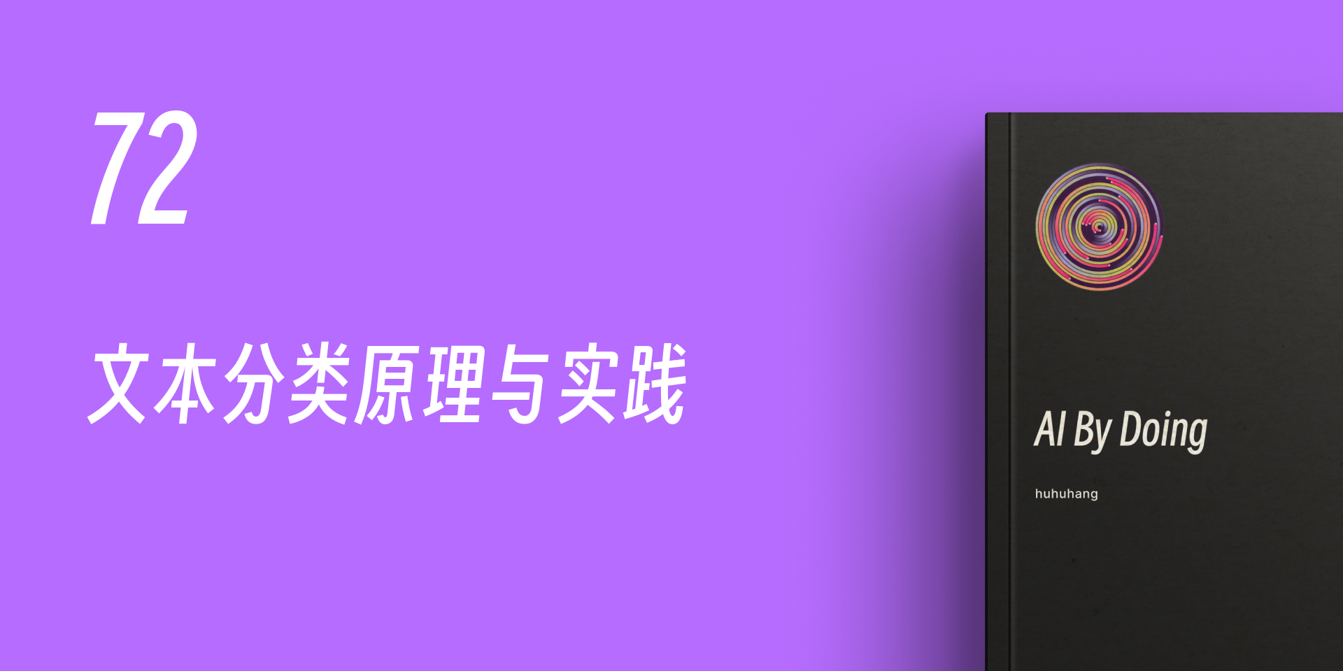
Bag of Words Model (English: Bag-of-words model, abbreviated as: BoW) is the most fundamental type of feature extraction method. Its main idea is to ignore the grammar and word order of the text and use an unordered sequence of words to represent a piece of text or a document. It can be understood in this way that we put all the words that appear in the entire document set into a bag, remove duplicates and arrange them in an unordered manner. In this way, the document can be represented according to the number of times the words appear.
Next, let’s demonstrate the steps of the bag-of-words model. For the following 3 English sentences (similarly for Chinese) shown in the figure below.
"The elephant sneezed at the sight of potatoes."
"Bats can see via echolocation. See the bat sight sneeze!"
"Wondering, she opened the door to the studio."
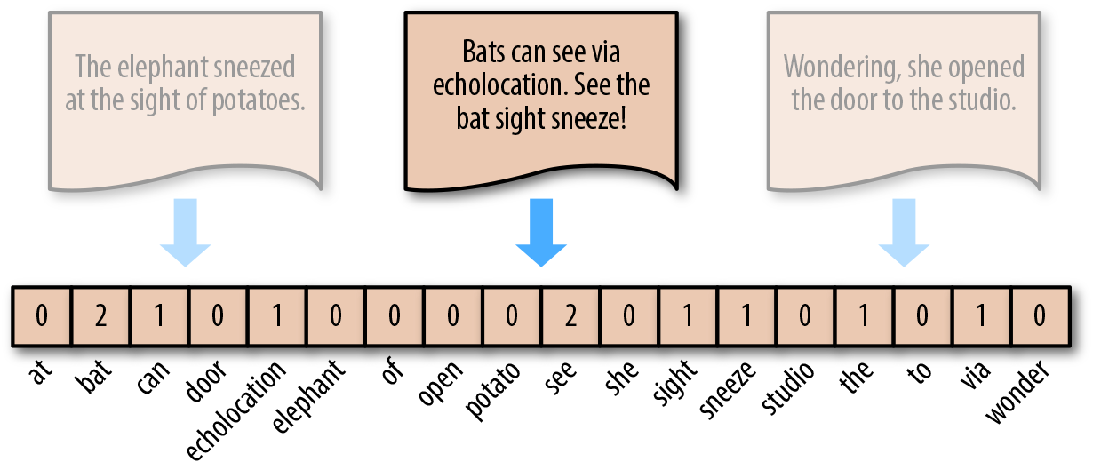
First, complete word segmentation → remove redundant punctuation characters → remove duplicates to obtain the words arranged horizontally as shown in the figure below, which is the bag of words. In English, singular and plural forms, as well as tenses, usually only retain the base form of the word.
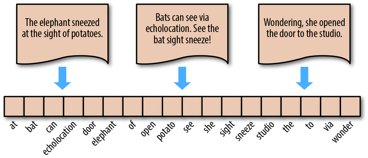
The representation method of the bag-of-words model is to count the number of occurrences of a certain word in the original sentence by referring to the bag of words. In this way, regardless of the length of the sentence, it can be represented by a bag-of-words vector of equal length. For example, for the sentence “Bats can see via echolocation. See the bat sight sneeze!”, it can be converted into the vector \([0, 2, 1, \cdots, 0, 1, 0]\).
We can use
sklearn.feature_extraction.text.CountVectorizer
provided by scikit - learn
🔗
to build a bag - of - words model. The method is very
simple and can be understood through the following
example.
from sklearn.feature_extraction.text import CountVectorizer

corpus = [
    "The elephant sneeze at the sight of potato.",
    "Bat can see via echolocation. See the bat sight sneeze!",
    "Wonder, she open the door to the studio.",
]

vectorizer = CountVectorizer()
vectors = vectorizer.fit_transform(corpus)
print(vectorizer.get_feature_names_out())  # 打印出词袋
vectors.toarray()  # 打印词向量
['at' 'bat' 'can' 'door' 'echolocation' 'elephant' 'of' 'open' 'potato'
 'see' 'she' 'sight' 'sneeze' 'studio' 'the' 'to' 'via' 'wonder']
array([[1, 0, 0, 0, 0, 1, 1, 0, 1, 0, 0, 1, 1, 0, 2, 0, 0, 0],
       [0, 2, 1, 0, 1, 0, 0, 0, 0, 2, 0, 1, 1, 0, 1, 0, 1, 0],
       [0, 0, 0, 1, 0, 0, 0, 1, 0, 0, 1, 0, 0, 1, 2, 1, 0, 1]])
In the above example, when creating the
corpus, we have manually processed the singular and plural
forms as well as the tense words in English words and
changed them all to the base form. This process can be
completed through preprocessing code in actual
applications.
Another small variant of the bag - of - words model is not to represent it by the actual number of occurrences of words, but to adopt a method similar to one - hot encoding. If a word appears, it is set to 1, and if it does not appear, it is 0.
This process can also be completed using scikit - learn.
Here,
sklearn.preprocessing.Binarizer
🔗
is used to perform one - hot encoding conversion on the
processing results of the above
CountVectorizer.
from sklearn.preprocessing import Binarizer

freq = CountVectorizer()
corpus_ = freq.fit_transform(corpus)

onehot = Binarizer()
onehot.fit_transform(corpus_.toarray())
array([[1, 0, 0, 0, 0, 1, 1, 0, 1, 0, 0, 1, 1, 0, 1, 0, 0, 0],
       [0, 1, 1, 0, 1, 0, 0, 0, 0, 1, 0, 1, 1, 0, 1, 0, 1, 0],
       [0, 0, 0, 1, 0, 0, 0, 1, 0, 0, 1, 0, 0, 1, 1, 1, 0, 1]])
73.5.2. TF-IDF Model#
TF-IDF Model (Term frequency–inverse document frequency) is a commonly used weighting technique for information retrieval and text mining. TF-IDF is a statistical method used to evaluate the importance of a word for a document collection or a single document in a corpus.
TF-IDF consists of two parts: TF (Term frequency) and IDF (Inverse document frequency). The calculation formula is:
In the formula, the numerator \(n_{ij}\) represents the frequency of the word \(i\) appearing in the document \(j\). The denominator is the sum of the frequencies of all words, that is, the total number of all words.
In the formula, \(\left | D \right |\) represents the total number of documents, and the denominator \(\left | D_{i} \right |\) represents the number of documents in the document set that contain the word \(i\). In the original formula, there is no \(+1\) in the denominator. Here, \(+1\) is used for Laplace smoothing to avoid the situation where the denominator becomes zero because some new words do not appear in the corpus.
Finally, multiplying the two values of TF and IDF can obtain the value of TF-IDF. That is:
Similarly, scikit-learn provides
sklearn.feature_extraction.text.TfidfVectorizer
🔗
which can be used for TF-IDF transformation.
from sklearn.feature_extraction.text import TfidfVectorizer

vectorizer = TfidfVectorizer()
tfidf = vectorizer.fit_transform(corpus)
tfidf.toarray()
array([[0.39066946, 0.        , 0.        , 0.        , 0.        ,
        0.39066946, 0.39066946, 0.        , 0.39066946, 0.        ,
        0.        , 0.29711419, 0.29711419, 0.        , 0.46147135,
        0.        , 0.        , 0.        ],
       [0.        , 0.56555816, 0.28277908, 0.        , 0.28277908,
        0.        , 0.        , 0.        , 0.        , 0.56555816,
        0.        , 0.21506078, 0.21506078, 0.        , 0.16701388,
        0.        , 0.28277908, 0.        ],
       [0.        , 0.        , 0.        , 0.36772387, 0.        ,
        0.        , 0.        , 0.36772387, 0.        , 0.        ,
        0.36772387, 0.        , 0.        , 0.36772387, 0.43436728,
        0.36772387, 0.        , 0.36772387]])
73.5.3. Word2Vec Model#
Word2Vec model is a vector representation method for words proposed by the Google team in 2015, also known as “word embedding”.
Whether it is the bag-of-words model or the TF-IDF model, they both use discrete vector values to represent text. These encodings are arbitrary and do not provide information about the possible relationships between words. Representing words as unique discrete values also leads to data sparsity and generally means that we may need more data to successfully train statistical models.
Vector space model represents (embeds) words in a continuous vector space, where semantically similar words are mapped to nearby points (embedded near each other). Vector space models have a long and rich history in NLP, but all methods rely in some way on the distributional hypothesis, which states that words that appear in the same context have the same semantics.

Word2Vec is a computationally efficient predictive model for learning word embeddings in raw text. It comes in two types: the Continuous Bag of Words model (CBOW) and the Skip-Gram model. Algorithmically, the two models are quite similar, except that CBOW predicts the target word (e.g., mat) from the source context words (the cat sits on the), while Skip-Gram does the reverse, predicting the source context words from the target word.
According to the paper, statistically, it helps CBOW organize a lot of distributional information. In most cases, this is very useful for small datasets. However, Skip-Gram treats each context-target pair as a new observation, and when we use large datasets, Skip-Gram seems to perform better. The specific explanation of the principle of Word2Vec is relatively complex. You can read the original paper or other relevant materials. In this experiment, we will focus on learning how to use Word2Vec.
The Word2Vec word embedding process is generally commonly
handled using the
Gensim
library. Gensim is a relatively commonly used tool in
natural language processing, which provides a packaged and
efficient Word2Vec processing class
gensim.modelsWord2Vec(). Its commonly used parameters are:
- vector_size: The dimension of the word embeddings, representing the length of the vector after each word is embedded.
- window: The maximum distance between the target word and the words around the target word.
- min_count: The minimum number of word occurrences to be considered when training the model. Words that appear less than this count will be ignored.
- sg: The training algorithm, CBOW(0) or Skip-Gram(1).
Next, we use Word2Vec to perform word embedding operations on the previous example text.
from gensim.models import Word2Vec

# 分词之后的示例文本
sentences = [
    ["the", "elephant", "sneeze", "at", "the", "sight", "of", "potato"],
    [
        "bat",
        "can",
        "see",
        "via",
        "echolocation",
        "see",
        "the",
        "bat",
        "sight",
        "sneeze",
    ],
    ["wonder", "she", "open", "the", "door", "to", "the", "studio"],
]

# 训练模型
model = Word2Vec(sentences, vector_size=20, min_count=1)
# 输出该语料库独立不重复词
print(list(model.wv.key_to_index))
# 输出 elephant 单词词嵌入后的向量
model.wv.get_vector("elephant")
['the', 'bat', 'sneeze', 'sight', 'see', 'elephant', 'at', 'of', 'potato', 'studio', 'to', 'via', 'echolocation', 'wonder', 'she', 'open', 'door', 'can']
array([-0.04309844,  0.01832869,  0.02594942,  0.02870969,  0.03733459,
       -0.03083838,  0.00552807,  0.03023641, -0.01420025, -0.03086761,
       -0.00205112, -0.04184474, -0.02800006,  0.03552269,  0.0167627 ,
        0.03612835,  0.03400124,  0.03765371, -0.01894577, -0.00280903],
      dtype=float32)
Next, we can plot the words after Word2Vec embedding in
space. Since the
vector_size=20
was set in the above model, we need to use PCA for
dimensionality reduction to reduce the embedded vectors to
two dimensions in order to visualize them in a plane.
from sklearn.decomposition import PCA
from matplotlib import pyplot as plt

%matplotlib inline

# PCA 降维
X = model.wv.vectors
pca = PCA(n_components=2)
result = pca.fit_transform(X)

# 绘制散点图,并将单词标记出来
plt.scatter(result[:, 0], result[:, 1])
words = list(model.wv.key_to_index)
for i, word in enumerate(words):
    plt.annotate(word, xy=(result[i, 0], result[i, 1]))

Since our corpus is small, the correlation between words is not very obvious. If the corpus is large enough, you can clearly see that some words with related meanings are closer in space.
Training a Word2Vec model often requires a large amount of corpus and time. Therefore, sometimes we use pre-trained word embedding models. For example, Google released a pre-trained Word2Vec model on the Word2Vec Project. This model was trained using Google News data (about 100 billion words), which contains 3 million words and phrases, and uses 300-dimensional word vectors for representation. Since the size of this pre-trained word embedding model is 3.4 GB, it will not be demonstrated here. You can download it locally and load the model using the following code.
from gensim.models import KeyedVectors

filename = 'GoogleNews-vectors-negative300.bin'
model = KeyedVectors.load_word2vec_format(filename, binary=True)
After obtaining the word embedding vectors for each word, we can get the vector features of a piece of text by directly summing or other weighted summation methods, and then these features can be passed into a classifier for training.
73.6. Fake News Classification Task#
So far, we have learned a series of preparatory work before text classification. Next, we will complete a real text classification task through an example.
WSDM - Fake News Classification is a competition on Kaggle. In this experiment, we use the dataset provided by it to complete a text classification task. First, download the dataset provided by the experiment.
wget -nc "https://cdn.aibydoing.com/aibydoing/files/wsdm_mini.csv"
--2023-11-14 10:39:05--  https://cdn.aibydoing.com/aibydoing/files/wsdm_mini.csv
正在解析主机 cdn.aibydoing.com (cdn.aibydoing.com)... 198.18.7.59
正在连接 cdn.aibydoing.com (cdn.aibydoing.com)|198.18.7.59|:443... 已连接。
已发出 HTTP 请求,正在等待回应... 200 OK
长度:2281530 (2.2M) [text/csv]
正在保存至: “wsdm_mini.csv”

wsdm_mini.csv       100%[===================>]   2.18M  3.10MB/s  用时 0.7s

2023-11-14 10:39:07 (3.10 MB/s) - 已保存 “wsdm_mini.csv” [2281530/2281530])
import pandas as pd

df = pd.read_csv("wsdm_mini.csv")
df.head()
| title1_zh | title2_zh | label | |
|---|---|---|---|
| 0 | 千叶湖八岁孩子不想去学英语,跳楼了 | 「辟谣」千叶湖八岁孩子跳楼了为谣言信息 | disagreed |
| 1 | 喝酸奶真的能补充益生菌吗? | 喝酸奶来补充益生菌,靠谱么? | agreed |
| 2 | 刚刚马云终于出手了!房价要跌,扬言房地产中介都要失业了 | 最新消息马云终于出手了!扬言房地产中介都要失业!6 | agreed |
| 3 | 直击“冯乡长”李正春追悼会:赵本山全程操办,赵四刘能现场祭奠 | 昆明会议直击“活摘”谣言 | unrelated |
| 4 | 李雨桐爆薛之谦离婚内幕,说到底就是网红之间的恩怨情仇嘛 | 薛之谦前女友李雨桐再次发微博爆料,薛之谦工作室发声明辟谣 | disagreed |
This dataset uses the training set provided by the original
competition, only retains the Chinese fields and samples
15,000 pieces of data. The dataset contains two feature
columns,
title1_zh
and
title2_zh, which are two news titles. The target value
label
represents the relationship between these two news, where:
-
agreed: B talks about the same fake news as A. -
disagreed: B refutes the fake news in A. -
unrelated: B has nothing to do with A.
There are 5,000 pieces of data for each of the 3 labels.
Following the idea in the above text, first we need to
tokenize the text. Before tokenization, first merge
title1_zh
and
title2_zh
into a single field
title_zh.
df['title_zh'] = df[['title1_zh', 'title2_zh']].apply(lambda x: ''.join(x), axis=1)  # 合并文本数据列
df_merge = df.drop(df.columns[[0, 1]], axis=1)  # 删除原文本列
df_merge.head()
| label | title_zh | |
|---|---|---|
| 0 | disagreed | 千叶湖八岁孩子不想去学英语,跳楼了「辟谣」千叶湖八岁孩子跳楼了为谣言信息 |
| 1 | agreed | 喝酸奶真的能补充益生菌吗?喝酸奶来补充益生菌,靠谱么? |
| 2 | agreed | 刚刚马云终于出手了!房价要跌,扬言房地产中介都要失业了最新消息马云终于出手了!扬言房地产中介... |
| 3 | unrelated | 直击“冯乡长”李正春追悼会:赵本山全程操办,赵四刘能现场祭奠昆明会议直击“活摘”谣言 |
| 4 | disagreed | 李雨桐爆薛之谦离婚内幕,说到底就是网红之间的恩怨情仇嘛薛之谦前女友李雨桐再次发微博爆料,薛之... |
Next, perform tokenization on
title_zh. Another important step in the tokenization process is
“removing stop words”. Generally speaking,
stop words
can be roughly divided into two categories. One category is
the function words in human language. These function words
are extremely common. Compared with other words, function
words have little practical meaning. For example,
the, is, at, which, on in English, and
的、得 in Chinese, etc. The other category
of words includes lexical words, such as high-frequency
words in large-scale corpora. Many high-frequency words can
only bring very little semantic information. Removing stop
words can improve the performance of subsequent text feature
extraction and classification.
Here, we can use the stop word dictionary provided in the course, which contains some meaningless common words and Chinese punctuation marks.
wget -nc "https://cdn.aibydoing.com/aibydoing/files/stopwords.txt" # 停用词词典
--2023-11-14 10:39:12--  https://cdn.aibydoing.com/aibydoing/files/stopwords.txt
正在解析主机 cdn.aibydoing.com (cdn.aibydoing.com)... 198.18.7.59
正在连接 cdn.aibydoing.com (cdn.aibydoing.com)|198.18.7.59|:443... 已连接。
已发出 HTTP 请求,正在等待回应... 200 OK
长度:未指定 [text/plain]
正在保存至: “stopwords.txt”

stopwords.txt           [ <=>                ]  12.98K  --.-KB/s  用时 0.09s

2023-11-14 10:39:13 (151 KB/s) - “stopwords.txt” 已保存 [13289]
Next, define a function to load the data in the stop word file.
def load_stopwords(file_path):
    with open(file_path, 'r') as f:
        stopwords = [line.strip('\n') for line in f.readlines()]
    return stopwords
stopwords = load_stopwords('stopwords.txt')
stopwords
Next comes the process of tokenization and stop word removal.
from tqdm.notebook import tqdm

corpus = []
for line in tqdm(df['title_zh']):
    words = []
    seg_list = list(jieba.cut(line))  # 分词
    for word in seg_list:
        if word in stopwords:  # 删除停用词
            continue
        words.append(word)
    corpus.append(words)
Next, we perform Word2Vec embedding on the words. At the same time, we add the vectors of each word in each piece of data as the final vector representation of the sentence.
import numpy as np

model = Word2Vec(corpus)  # 词嵌入,默认 size=100

def sum_vec(text):
    vec = np.zeros(100).reshape((1, 100))  # 初始化一个和 Word2Vec 嵌入等长度的 0 向量
    for word in text:
        # 得到句子中每个词的词向量并累加在一起
        if word in list(model.wv.index_to_key):
            vec += model.wv.get_vector(word).reshape((1, 100))
        else:
            pass
    return vec

# 将词向量保存为 Ndarray
X = np.concatenate([sum_vec(z) for z in tqdm(corpus)])
X.shape
(15000, 100)
Currently, having completed feature extraction, we can start building a classifier and training a text classification model in the conventional way.
from sklearn.model_selection import train_test_split
from sklearn.ensemble import RandomForestClassifier

X_train, X_test, y_train, y_test = train_test_split(X, df.label, test_size=0.2)
clf = RandomForestClassifier()
clf.fit(X_train, y_train)
clf.score(X_test, y_test)
0.6583333333333333
At this point, we can obtain the accuracy of text classification. Of course, you may find that the results are not very satisfactory. In fact, this may be due to the small amount of data, which affects the effect of word embedding. At the same time, simply performing text classification in this fake news classification competition cannot achieve particularly good results.
73.7. Summary#
In this experiment, we learned about the text classification task in natural language processing. Among them, we focused on learning Chinese and English word segmentation, as well as common feature extraction models. These two tasks are the key to completing text classification and require a full understanding of them. Although we have already come into contact with some knowledge of text classification in the previous study of recurrent neural networks, this experiment provides a more detailed introduction to the preprocessing link of text classification, and you can have a second understanding in combination with the previous experiments.
Related Links