Pro Membership

Pro Membership is a membership plan created by the author to maintain and update this tutorial. You can get more benefits and services, click to view details.

72. LSTM Prediction of Stock Prices

72.1. Introduction

Stock trading trend prediction is one of the tasks involved in quantitative trading, that is, to analyze and predict price trends through statistical and machine learning methods. Generally, we can use time series related modeling methods, but in this challenge, we will try to use LSTM to complete stock prediction analysis.

72.2. Key Points

• LSTM Network Construction

• Stock Price Prediction

I believe every stock investor hopes to predict stock prices and profit from the stock market with the ability to foretell the future. Since there are many factors affecting stock price changes and most of these factors are not quantifiable, this is an extremely difficult task.

However, if we regard the historical stock data as a time series, we can analyze the trend changes through time series modeling in statistics. In addition, the recurrent neural network also performs well for sequence models. Therefore, in this challenge, we will use the LSTM network to predict the stock price trend.

First, we obtain the trading data of real-time stocks. Here, we choose the Quandl financial data module. For this challenge, it is necessary to install the Python library provided by Quandl first.

{note}
pip install quandl

Unregistered users of Quandl can submit 50 access requests per day, while there is no limit for registered accounts. For this experiment, we use the test account provided by the course. If you use it by yourself, please obtain the API KEY by registering for free through the official website.

import quandl

# 该 API KEY 仅限课程使用，其他用途请自行注册
quandl.ApiConfig.api_key = 'DdXEs2xFciyUXrER9-a7'
# 获取苹果公司股票数据
df_aapl = quandl.get('WIKI/AAPL')
df_aapl.head()

	Open	High	Low	Close	Volume	Ex-Dividend	Split Ratio	Adj. Open	Adj. High	Adj. Low	Adj. Close	Adj. Volume
Date
1980-12-12	28.75	28.87	28.75	28.75	2093900.0	0.0	1.0	0.422706	0.424470	0.422706	0.422706	117258400.0
1980-12-15	27.38	27.38	27.25	27.25	785200.0	0.0	1.0	0.402563	0.402563	0.400652	0.400652	43971200.0
1980-12-16	25.37	25.37	25.25	25.25	472000.0	0.0	1.0	0.373010	0.373010	0.371246	0.371246	26432000.0
1980-12-17	25.87	26.00	25.87	25.87	385900.0	0.0	1.0	0.380362	0.382273	0.380362	0.380362	21610400.0
1980-12-18	26.63	26.75	26.63	26.63	327900.0	0.0	1.0	0.391536	0.393300	0.391536	0.391536	18362400.0

df_aapl.tail()

	Open	High	Low	Close	Volume	Ex-Dividend	Split Ratio	Adj. Open	Adj. High	Adj. Low	Adj. Close	Adj. Volume
Date
2018-03-21	175.04	175.09	171.26	171.270	35247358.0	0.0	1.0	175.04	175.09	171.26	171.270	35247358.0
2018-03-22	170.00	172.68	168.60	168.845	41051076.0	0.0	1.0	170.00	172.68	168.60	168.845	41051076.0
2018-03-23	168.39	169.92	164.94	164.940	40248954.0	0.0	1.0	168.39	169.92	164.94	164.940	40248954.0
2018-03-26	168.07	173.10	166.44	172.770	36272617.0	0.0	1.0	168.07	173.10	166.44	172.770	36272617.0
2018-03-27	173.68	175.15	166.92	168.340	38962839.0	0.0	1.0	173.68	175.15	166.92	168.340	38962839.0

Through the above code, we can load the historical trading data of Apple since its listing. Since real-time data requires a paid subscription, we can only obtain free data with an earlier cut-off date.

For this challenge, we only use the historical data of Apple after 2010 and specify the adjusted closing price (Adj. Close) as the prediction target. Next, we first plot the change curve of the closing price.

from matplotlib import pyplot as plt
from pandas.plotting import register_matplotlib_converters
%matplotlib inline
register_matplotlib_converters()

df = df_aapl['2010':]["Adj. Close"]
plt.plot(df)

[<matplotlib.lines.Line2D at 0x129465630>]

Then, for this challenge, the data before 2018 is used as training data, and the data after 2018 is used as test data. At the same time, we normalize the data.

import numpy as np
from sklearn.preprocessing import MinMaxScaler

df_train = df[:'2018']  # 训练数据
df_test = df['2018':]  # 测试数据

scaler = MinMaxScaler(feature_range=(0, 1))  # 归一化
df_train_scaler = scaler.fit_transform(df_train.values.reshape(-1, 1))
df_test_scaler = scaler.transform(df_test.values.reshape(-1, 1))

df_train_scaler.shape, df_test_scaler.shape

((2070, 1), (59, 1))

Since MinMaxScaler must be passed a two-dimensional array, .reshape(-1, 1) is used above to transform the shape of the data.

Next, we need to design an experimental plan. Here, we adopt the strategy of predicting tomorrow based on today, with a time interval of 1 day. Therefore, the time series needs to be shifted by 1 day for correspondence.

time_step = 1

train_t0 = df_train_scaler[:-time_step]  # 训练数据错位 1 天
train_t1 = df_train_scaler[time_step:]

test_t0 = df_test_scaler[:-time_step]
test_t1 = df_test_scaler[time_step:]

As shown above, when the t0 sequence and the t1 sequence are corresponding, there is a 1-day time shift. Therefore, we can use train_t0 as the input to the network, while train_t1 is used as the target value to train the LSTM network.

Exercise 72.1

Challenge: Build an LSTM model using the TensorFlow Keras sequential model building method.

Requirement: Define the model structure with reference to the expected output.

import tensorflow as tf

## 代码开始 ### (≈ 4 行代码)
model = None
## 代码结束 ###

Solution to Exercise 72.1

import tensorflow as tf

### Code starts ### (≈ 4 lines of code)
model = tf.keras.Sequential()
model.add(tf.keras.layers.LSTM(32, input_shape=(1, 1), return_sequences=True))
model.add(tf.keras.layers.LSTM(16))
model.add(tf.keras.layers.Dense(1))
### Code ends ###

Run the test

model.summary()

Expected output:

_________________________________________________________________
Layer (type)                 Output Shape              Param #   
=================================================================
lstm_1 (LSTM)                (None, 1, 32)             4352      
_________________________________________________________________
lstm_2 (LSTM)                (None, 16)                3136      
_________________________________________________________________
dense_1 (Dense)              (None, 1)                 17        
=================================================================
Total params: 7,505
Trainable params: 7,505
Non-trainable params: 0
_________________________________________________________________

Next, compile and train the model.

Exercise 72.2

Challenge: Compile and train the LSTM model defined above.

Requirement: Freely choose the parameters.

## 代码开始 ### (≈ 2 行代码)

## 代码结束 ###

Solution to Exercise 72.2

### Code starts ### (≈ 2 lines of code)
model.compile(loss='mse', optimizer='adam')
model.fit(np.atleast_3d(train_t0),
          train_t1.reshape(-1), epochs=5, batch_size=32)
### Code ends ###

Finally, use test_t0 for testing and calculate the MAPE value between it and test_t1. At the same time, the challenge requires plotting the real data change curve and the predicted structure change curve on the same graph for comparison. Since the data used for prediction is the normalized result, you can use the inverse_transform method provided by MinMaxScaler to restore the data.

Exercise 72.3

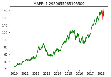
Challenge: Test and plot a comparison image of the real and predicted results.

Requirement: Show the real results as green lines and the predicted results as red lines, referring to the expected output style.

## 代码开始 ### (> 10 行代码)

## 代码结束 ###

Solution to Exercise 72.3

test_pred = model.predict(np.atleast_3d(test_t0))  # Predict the test data
test_pred = scaler.inverse_transform(test_pred)  # Restore the data

# Replace the prediction part in the original data format and set the training part data as NAN for easy plotting on the same graph
df_pred = df.copy()
df_pred[len(df_pred)-len(test_pred):] = test_pred.reshape(-1)
df_pred[:-len(test_pred)] = np.nan

# Calculate the MAPE result
def mape(y_true, y_pred):
    n = len(y_true)
    mape = 100 * np.sum(np.abs((y_true-y_pred)/y_true)) / n
    return mape


y_true = df[len(df_pred)-len(test_pred):].values
y_pred = test_pred.reshape(-1)
mape = mape(y_true, y_pred)

plt.plot(df, 'g')
plt.plot(df_pred, 'r')
plt.title(f"MAPE: {mape}")

Expected output:

---

○ Sharethis article link to your social media, blog, forum, etc. More external links will increase the search engine ranking of this site.

If you find this content helpful, you can buy me a coffee

Previous

71. Construction of Recurrent Neural Networks

Next

73. Text Classification Principles and Practices