
71. Construction of Recurrent Neural Networks#
71.1. Introduction#
In the previous experiments, we learned about Recurrent Neural Networks (RNNs). RNNs are widely used in natural language processing, speech recognition, and other fields. Their “memory” ability has great advantages in processing sequence models. In this lesson, we will learn how to build and train RNNs using deep learning frameworks.
71.2. Key Points#
IMDB Dataset
Word Embedding
Simple Recurrent Neural Network
LSTM Recurrent Neural Network
Previously, we introduced the concept of recurrent neural
networks. We also understood simple recurrent neural
networks and common LSTM network structures, GRU network
structures, etc. through pictures and examples. Implementing
a network structure like LSTM using low-level APIs is still
relatively complex, so this experiment mainly uses
high-level APIs such as
tf.keras
to complete.
In addition, when building recurrent neural networks, it is inevitable to come into contact with some natural language-related terms and knowledge points. You need to consult more materials to help with understanding. In the subsequent course content, there will also be in-depth learning related to natural language processing.
71.3. IMDB Dataset#
Like many datasets we have encountered before, the IMDB dataset is a very popular benchmark dataset, and many papers use it to test the performance of algorithms. The IMDB data is sourced from the famous Internet Movie Database IMDB.COM.

This dataset contains a total of 50,000 review data points, which are labeled as positive (1) or negative (0). Each review in the dataset has been preprocessed and encoded as a sequence representation of word indices (integers). The word index means that words are indexed according to their frequency of occurrence in the dataset. For example, the integer 3 encodes the third most frequent word in the data. Generally, the IMDB dataset is split into a training set and a test set, each accounting for half. When the Stanford researchers released this dataset in 2011, the achieved prediction accuracy was 88.89%.
import numpy as np
import tensorflow as tf

# 加载数据, num_words 表示只考虑最常用的 n 个词语,代表本次所用词汇表大小
MAX_DICT = 1000
(X_train, y_train), (X_test, y_test) = tf.keras.datasets.imdb.load_data(
    num_words=MAX_DICT
)

X_train.shape, y_train.shape, X_test.shape, y_test.shape
Downloading data from https://storage.googleapis.com/tensorflow/tf-keras-datasets/imdb.npz
17464789/17464789 [==============================] - 1s 0us/step
((25000,), (25000,), (25000,), (25000,))
As can be seen, there are 25,000 data points in both the
training set and the test set. Next, output
X_train[0]
to view the first review:
np.array(X_train[0]) # 直接运行
array([  1,  14,  22,  16,  43, 530, 973,   2,   2,  65, 458,   2,  66,
         2,   4, 173,  36, 256,   5,  25, 100,  43, 838, 112,  50, 670,
         2,   9,  35, 480, 284,   5, 150,   4, 172, 112, 167,   2, 336,
       385,  39,   4, 172,   2,   2,  17, 546,  38,  13, 447,   4, 192,
        50,  16,   6, 147,   2,  19,  14,  22,   4,   2,   2, 469,   4,
        22,  71,  87,  12,  16,  43, 530,  38,  76,  15,  13,   2,   4,
        22,  17, 515,  17,  12,  16, 626,  18,   2,   5,  62, 386,  12,
         8, 316,   8, 106,   5,   4,   2,   2,  16, 480,  66,   2,  33,
         4, 130,  12,  16,  38, 619,   5,  25, 124,  51,  36, 135,  48,
        25,   2,  33,   6,  22,  12, 215,  28,  77,  52,   5,  14, 407,
        16,  82,   2,   8,   4, 107, 117,   2,  15, 256,   4,   2,   7,
         2,   5, 723,  36,  71,  43, 530, 476,  26, 400, 317,  46,   7,
         4,   2,   2,  13, 104,  88,   4, 381,  15, 297,  98,  32,   2,
        56,  26, 141,   6, 194,   2,  18,   4, 226,  22,  21, 134, 476,
        26, 480,   5, 144,  30,   2,  18,  51,  36,  28, 224,  92,  25,
       104,   4, 226,  65,  16,  38,   2,  88,  12,  16, 283,   5,  16,
         2, 113, 103,  32,  15,  16,   2,  19, 178,  32])
As can be seen, what is output are word indices. Then, if you want to see the original review content, you need to find the original words from the dictionary through the indices, which can be done with the following code:
index = tf.keras.datasets.imdb.get_word_index()  # 获取词索引表
reverse_index = dict([(value, key) for (key, value) in index.items()])
comment = " ".join([reverse_index.get(i - 3, "#") for i in X_train[0]])  # 还原第 1 条评论
comment
Downloading data from https://storage.googleapis.com/tensorflow/tf-keras-datasets/imdb_word_index.json
1641221/1641221 [==============================] - 1s 0us/step
"# this film was just brilliant casting # # story direction # really # the part they played and you could just imagine being there robert # is an amazing actor and now the same being director # father came from the same # # as myself so i loved the fact there was a real # with this film the # # throughout the film were great it was just brilliant so much that i # the film as soon as it was released for # and would recommend it to everyone to watch and the # # was amazing really # at the end it was so sad and you know what they say if you # at a film it must have been good and this definitely was also # to the two little # that played the # of # and paul they were just brilliant children are often left out of the # # i think because the stars that play them all # up are such a big # for the whole film but these children are amazing and should be # for what they have done don't you think the whole story was so # because it was true and was # life after all that was # with us all"
When initially loading the dataset, we set
num_words
                      =
                      1000
, which means the dataset only contains a dictionary of
1000 common words. Therefore, in the above output statement,
some of the words replaced by # are not among these 1000
common words.
If you output multiple reviews, you will find that the lengths of each review are different. However, when inputting into the neural network, we must ensure that the shape of each piece of data is consistent. Therefore, preprocessing of the data is required here.
Here, we use
tf.keras.preprocessing.sequence.pad_sequences()
🔗
for processing. By specifying the maximum length
maxlen, we achieve the purpose of trimming the vectors. At the
same time, if the original sentence length is insufficient,
it will be padded with 0s at the beginning.
MAX_LEN = 200  # 设定句子最大长度
X_train = tf.keras.preprocessing.sequence.pad_sequences(X_train, MAX_LEN)
X_test = tf.keras.preprocessing.sequence.pad_sequences(X_test, MAX_LEN)

X_train.shape, X_test.shape
((25000, 200), (25000, 200))
At this time, you can see that each sentence has been forced to be processed into the specified length.
As we all know, machines cannot understand natural language like humans, so we need to convert the statements into tensors. During the above preprocessing process, each word has been converted into a number by the “dictionary”, and the sentences have also been represented in the form of word indices. So, can we directly input them into the neural network?
The answer is of course yes. However, based on experience, such a simple dictionary conversion often doesn’t work well. So generally, other means are introduced to further process the word indices.
71.4. Word Embedding#
Word Embedding, which is called “词嵌入” in Chinese, is a very commonly used method for characteristically processing word indices.
Regarding Embedding, here is a simple example to help understand. For instance, the word index corresponding to the word “apple” is 100. After being transformed by Embedding, 100 can be turned into a vector of a specified size, such as being transformed into \([1, 2, 1]\). Among them, 1 indicates that an apple is a very likable thing, 2 indicates that an apple is a fruit, and the last 1 indicates that an apple is beneficial to health. This is a process of characterization.
A dictionary can only simply process words into numerical values, but Embedding can directly establish connections between words. For example, “orange” may be closer in space to “apple” because they share the same fruit characteristics. As the following example shows, Embedding can freely group semantically similar items together and separate dissimilar items. For example, countries and their capitals, men and women.

Regarding word embeddings, there will be further
explanations in subsequent experiments. The Embedding layer
tf.keras.layers.Embedding
in Keras
🔗
can help us quickly complete the Embedding process.
tf.keras.layers.Embedding(input_dim, output_dim, embeddings_initializer='uniform', embeddings_regularizer=None, activity_regularizer=None, embeddings_constraint=None, mask_zero=False, input_length=None)
- input_dim: int > 0, the size of the vocabulary.
- output_dim: int >= 0, the dimension of the word vectors.
- input_length: the length of the input sequences when it is fixed. This argument is required if you need to connect Flatten and Dense layers.
With the Embedding structure, we can build a simple fully-connected network to complete comment sentiment classification.
model = tf.keras.Sequential()
model.add(tf.keras.layers.Embedding(MAX_DICT, 16, input_length=MAX_LEN))
model.add(tf.keras.layers.Flatten())
model.add(tf.keras.layers.Dense(1, activation="sigmoid"))

model.summary()
Model: "sequential"
_________________________________________________________________
 Layer (type)                Output Shape              Param #
=================================================================
 embedding (Embedding)       (None, 200, 16)           16000

 flatten (Flatten)           (None, 3200)              0

 dense (Dense)               (None, 1)                 3201

=================================================================
Total params: 19201 (75.00 KB)
Trainable params: 19201 (75.00 KB)
Non-trainable params: 0 (0.00 Byte)
_________________________________________________________________
In the above model,
input_dim=
is passed the previously set value of the vocabulary. When
connecting the Flatten layer later,
input_length=
is specified according to the requirements of the document,
that is, the length after the input sequence is forcibly
truncated.
The model requires a loss function and an optimizer during
training. Since this is a binary classification problem and
the model outputs a probability (a single-unit layer with a
sigmoid activation function), we will use the
binary_crossentropy
binary cross-entropy loss function.
model.compile(optimizer="Adam", loss="binary_crossentropy", metrics=["accuracy"])
Finally, complete iterative training and evaluation.
EPOCHS = 1
BATCH_SIZE = 64
model.fit(X_train, y_train, BATCH_SIZE, EPOCHS, validation_data=(X_test, y_test))
391/391 [==============================] - 1s 1ms/step - loss: 0.5799 - accuracy: 0.6917 - val_loss: 0.3916 - val_accuracy: 0.8359
<keras.src.callbacks.History at 0x28f2a56c0>
71.5. Simple Recurrent Neural Network#
A simple recurrent neural network is a fully connected RNN
where the output is fed back into the input. In TensorFlow,
it can be directly implemented by calling
tf.keras.layers.SimpleRNN
🔗.
tf.keras.layers.SimpleRNN(units, activation='tanh', use_bias=True, kernel_initializer='glorot_uniform', recurrent_initializer='orthogonal', bias_initializer='zeros', kernel_regularizer=None, recurrent_regularizer=None, bias_regularizer=None, activity_regularizer=None, kernel_constraint=None, recurrent_constraint=None, bias_constraint=None, dropout=0.0, recurrent_dropout=0.0, return_sequences=False, return_state=False, go_backwards=False, stateful=False, unroll=False)
- units: Positive integer, dimensionality of the output space.
- activation: Activation function to use. If you pass None, no activation is applied (ie. "linear" activation: a(x) = x).
- use_bias: Boolean, whether the layer uses a bias vector.
- dropout: Float between 0 and 1.
- return_sequences: Boolean. Whether to return the last output in the output sequence, or the full sequence.
Here, let’s explain the meaning of the parameter
dropout. In fact, Dropout is a concept often encountered in deep
learning, and it often appears as a network layer like
tf.keras.layers.Dropout
🔗. The main role of Dropout is to prevent overfitting. Its
principle of implementation is to disconnect the connections
between neurons with a certain probability (the Dropout
parameter value). In addition, for
return_sequences, you can read:
Understanding Two Important Parameters of the LSTM Layer
in Keras.
Next, start building a sequential model structure using Keras. This recurrent neural network consists of three layers: Embedding, SimpleRNN, and a Dense fully connected layer for output.
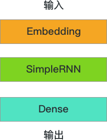
The code is as follows:
model_RNN = tf.keras.Sequential()
model_RNN.add(tf.keras.layers.Embedding(MAX_DICT, 32))
# dropout 是层与层之前的 dropout 数值,recurrent_dropout 是上个时序与这个时序的 dropout 值
model_RNN.add(tf.keras.layers.SimpleRNN(units=32, dropout=0.2, recurrent_dropout=0.2))
model_RNN.add(tf.keras.layers.Dense(1, activation="sigmoid"))

model_RNN.summary()
Model: "sequential_1"
_________________________________________________________________
 Layer (type)                Output Shape              Param #
=================================================================
 embedding_1 (Embedding)     (None, None, 32)          32000

 simple_rnn (SimpleRNN)      (None, 32)                2080

 dense_1 (Dense)             (None, 1)                 33

=================================================================
Total params: 34113 (133.25 KB)
Trainable params: 34113 (133.25 KB)
Non-trainable params: 0 (0.00 Byte)
_________________________________________________________________
model_RNN.summary()
can help us clearly see the model structure, and the total
number of parameters the model has to learn is relatively
large. Next, we compile and train the model, and finally
output the evaluation of the model on the test set.
model_RNN.compile(optimizer="Adam", loss="binary_crossentropy", metrics=["accuracy"])
model_RNN.fit(X_train, y_train, BATCH_SIZE, EPOCHS, validation_data=(X_test, y_test))
391/391 [==============================] - 12s 31ms/step - loss: 0.7037 - accuracy: 0.5177 - val_loss: 0.6864 - val_accuracy: 0.5347
<keras.src.callbacks.History at 0x28bc3d300>
For the analysis of the model accuracy, please refer to the latter part of the experiment.
71.6. Long Short-Term Memory (LSTM) Recurrent Neural Network#
Next, we replace the above SimpleRNN structure with an LSTM
structure, which can be directly implemented by calling
tf.keras.layers.LSTM
🔗
in TensorFlow. The API parameters are almost the same as
those of SimpleRNN, so we won’t go into details here.
model_LSTM = tf.keras.Sequential()
model_LSTM.add(tf.keras.layers.Embedding(MAX_DICT, 32))
model_LSTM.add(tf.keras.layers.LSTM(units=32, dropout=0.2, recurrent_dropout=0.2))
model_LSTM.add(tf.keras.layers.Dense(1, activation="sigmoid"))

model_LSTM.summary()
Model: "sequential_2"
_________________________________________________________________
 Layer (type)                Output Shape              Param #
=================================================================
 embedding_2 (Embedding)     (None, None, 32)          32000

 lstm (LSTM)                 (None, 32)                8320

 dense_2 (Dense)             (None, 1)                 33

=================================================================
Total params: 40353 (157.63 KB)
Trainable params: 40353 (157.63 KB)
Non-trainable params: 0 (0.00 Byte)
_________________________________________________________________
From the output of
model_LSTM.summary(), we can see that LSTM learns some additional parameters
compared to the simple RNN, but these parameters help us
avoid fatal problems such as the vanishing gradient. We keep
the other neural network layers unchanged, and the two
dropout values of LSTM are the same as those of SimpleRNN.
Next, start training the LSTM network. Since there are more parameters, the overall training time will be significantly longer than before.
model_LSTM.compile(optimizer="Adam", loss="binary_crossentropy", metrics=["accuracy"])
model_LSTM.fit(X_train, y_train, BATCH_SIZE, EPOCHS, validation_data=(X_test, y_test))
391/391 [==============================] - 39s 98ms/step - loss: 0.4891 - accuracy: 0.7540 - val_loss: 0.3546 - val_accuracy: 0.8464
<keras.src.callbacks.History at 0x28832dbd0>
It can be observed that the accuracy of LSTM on the test set is slightly higher than that of SimpleRNN. As a module of the recurrent neural network, LSTM is very cleverly designed. By continuously updating the memory cells through the forget gate and the input gate, it eliminates the fatal problem of gradient vanishing during the training of the recurrent neural network, and thus has been widely used.
Finally, we simply modify the code to replace the previous LSTM layer with a GRU layer. The GRU structure learns fewer parameters compared to LSTM, but the accuracy may not necessarily be better.
model_GRU = tf.keras.Sequential()
model_GRU.add(tf.keras.layers.Embedding(MAX_DICT, 32))
model_GRU.add(tf.keras.layers.GRU(units=32, dropout=0.2, recurrent_dropout=0.2))
model_GRU.add(tf.keras.layers.Dense(1, activation="sigmoid"))

model_GRU.summary()
Model: "sequential_3"
_________________________________________________________________
 Layer (type)                Output Shape              Param #
=================================================================
 embedding_3 (Embedding)     (None, None, 32)          32000

 gru (GRU)                   (None, 32)                6336

 dense_3 (Dense)             (None, 1)                 33

=================================================================
Total params: 38369 (149.88 KB)
Trainable params: 38369 (149.88 KB)
Non-trainable params: 0 (0.00 Byte)
_________________________________________________________________
model_GRU.compile(optimizer="Adam", loss="binary_crossentropy", metrics=["accuracy"])
model_GRU.fit(X_train, y_train, BATCH_SIZE, EPOCHS, validation_data=(X_test, y_test))
391/391 [==============================] - 34s 84ms/step - loss: 0.5066 - accuracy: 0.7357 - val_loss: 0.3934 - val_accuracy: 0.8260
<keras.src.callbacks.History at 0x28d5b3a90>
Finally, let’s discuss the issue of the evaluation accuracy of the test set in this experiment.
Above, we have respectively built four models: the fully connected network, SimpleRNN, LSTM, and GRU. You may find that in many cases, the recurrent neural network does not perform as well as the fully connected network, especially SimpleRNN. Isn’t it said that the recurrent neural network is very good at natural language processing? In fact, due to the large number of parameters involved in the recurrent neural network, there may be some small tricks in its training. For example, there is a discussion on Zhihu about What special tricks do you have when training RNN. This requires you to have an in-depth understanding of the network and application experience to be familiar with it.
In addition, Francois Chollet (the founder of Keras) once said that recurrent neural networks such as LSTM are less helpful for sentiment analysis problems. Although this statement is debatable, on the IMDB dataset, the performance of LSTM does indeed seem unsatisfactory. This should also be one of the reasons for the low accuracy of the test set.
Finally, the experiment provides a solution idea to improve the accuracy of IMDB classification. This solution uses TFIDF + Logistic Regression. TFIDF is a feature extraction method, and finally achieved an accuracy of 89% on the test set. Those who are interested can view the source code through GitHub.
71.7. Summary#
In this experiment, we mainly learned how to use the
high-level APIs provided by
tf.keras
to build recurrent neural network models.
tf.keras
provides common recurrent neural network structures such as
SimpleRNN, LSTM, and GRU, which are the preferred solutions
in general cases. Although recurrent neural networks do not
have obvious advantages in some specific problems, their
role cannot be underestimated. Later, as we deepen our study
of natural language processing, you will gradually see some
very good examples of recurrent neural networks.