
68. Object Detection Principles and Practices#
68.1. Introduction#
In addition to image classification, image generation, and image denoising, object detection is also a very common type of problem in the field of computer vision, with wide applications in face detection, pedestrian detection, image retrieval, and video surveillance. In fact, the concept of image classification is often used in object detection as well. In this experiment, we will learn what object detection is, as well as the methods and applications of object detection.
68.2. Key Points#
Object Detection Methods
R-CNN Family
YOLO and SSD
Mask R-CNN
TensorFlow Object Detection
Object detection, also known as object detection or object recognition in English, is simply put, a computer technology related to computer vision and image processing. It involves detecting instances of semantic objects of specific classes (such as people, buildings, or cars) in digital images and videos. Object detection has a wide range of applications in computer vision fields such as face detection, pedestrian detection, image retrieval, and video surveillance. Detecting and recognizing dynamic objects is also a key technology that needs to be overcome in autonomous driving.
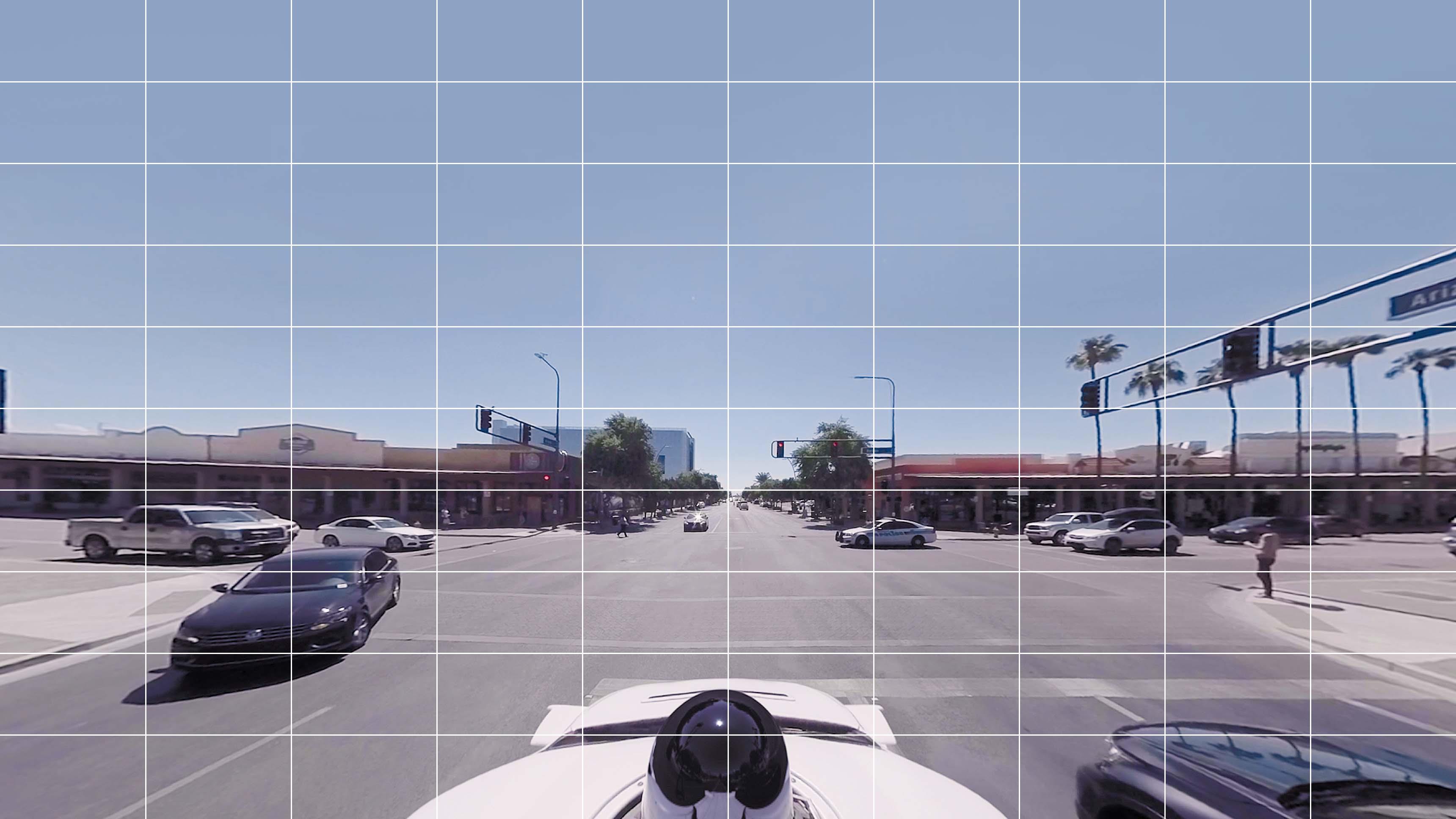
Before formally learning object detection methods, we first need to try to understand what object detection is. Now, suppose we build a road condition detection system for an autonomous vehicle. At this time, the autonomous vehicle captures the picture shown below. How would you describe this picture?

There are other cars in motion, pedestrians preparing to cross the road, and traffic lights in the picture. Since the traffic signs are not clearly visible, the road condition detection system of the car should accurately identify the positions where people are walking, the positions of other vehicles, and the colors of the traffic lights so that we can plan the correct route.
So what can the road condition detection system do? Generally speaking, what it can do is to create a bounding box around the objects so that the system can determine the positions of people, cars and other objects in the image, and then decide which path to take accordingly to avoid any accidents.
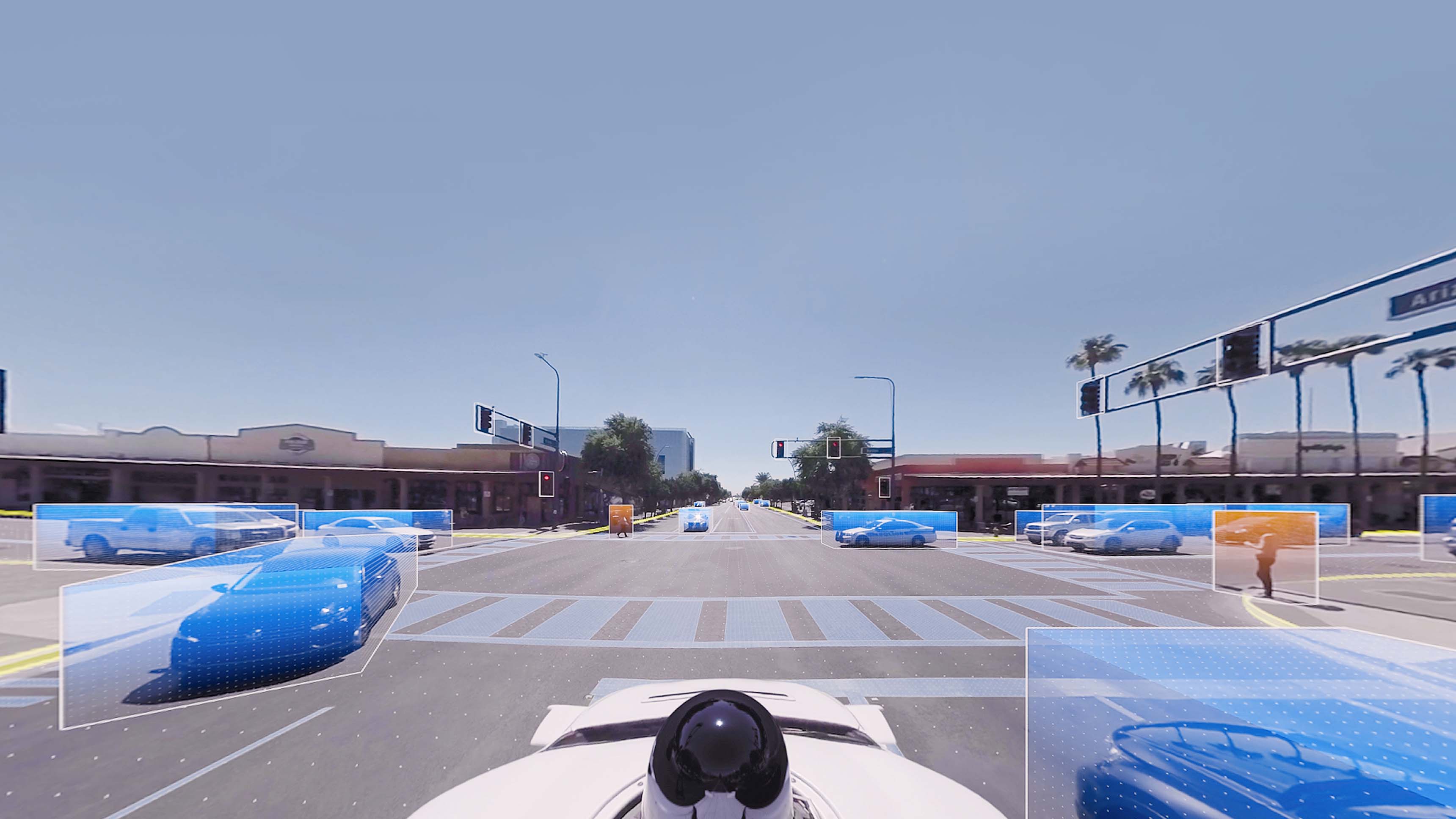
So, object detection actually mainly does one thing. Identify all the objects that are specified to exist in the image and their positions, and mark them out.
68.3. Object Detection Methods#
Next, we start to learn about the methods commonly used in object detection. Here, we start from the most basic. The simplest method that can be adopted here is to divide the image into four parts:
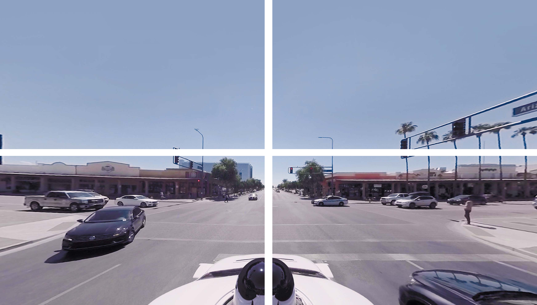
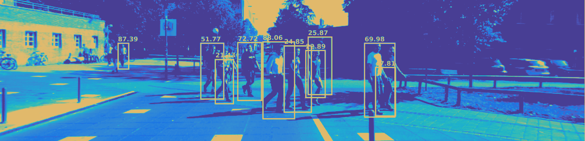
Next, each of the divided parts is provided to an image classifier, which will tell us whether the image contains a pedestrian. If so, that part can be marked out using a bounding box.
Intuitively, you all know that doing this is inaccurate. If autonomous driving adopts the above method, it will basically be a road hazard. Of course, you may think of improving it by increasing the number of segments, but just doing this is still not enough.
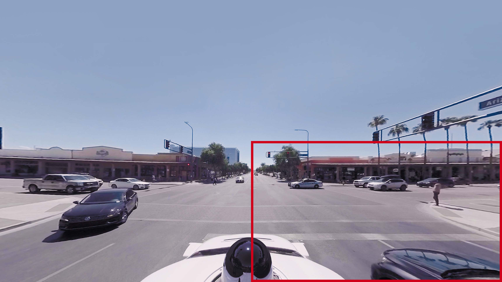
Later on, structured partitioning methods are still used to improve the accuracy of object detection. For example, we can divide the image into a \(10×10\) grid.
At this time, for each grid, we can try to extract slices containing different numbers of adjacent grids centered on it and finally submit them to the classifier.
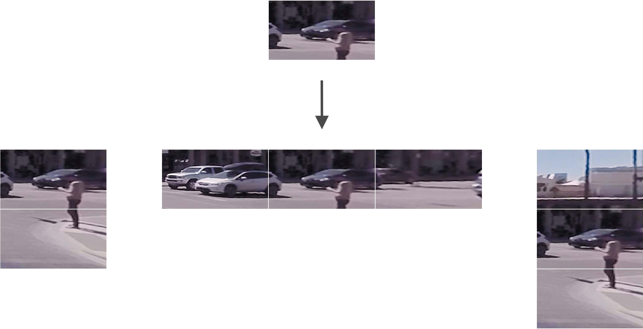
Then the classifier gives the slice with the highest accuracy and the smallest area to frame the target object.

It seems to have a good effect. So, is it possible to continue to improve? Of course. If the grid size is increased at this time and more slices with different heights and aspect ratios are extracted, the calibration of the red box will surely be more accurate. However, it can be imagined that the time complexity of the above method is too high.
With the rapid development of deep learning, the means and methods of object detection are also rapidly iterating. Currently, there are already a large number of methods that use deep learning for feature selection and build end-to-end methods, which use deep neural networks to make more rigorous and refined bounding box predictions. Next, through a graphical introduction that does not involve mathematical operations, we will take you to quickly understand the object detection methods related to deep learning.
68.3.1. R-CNN Family#
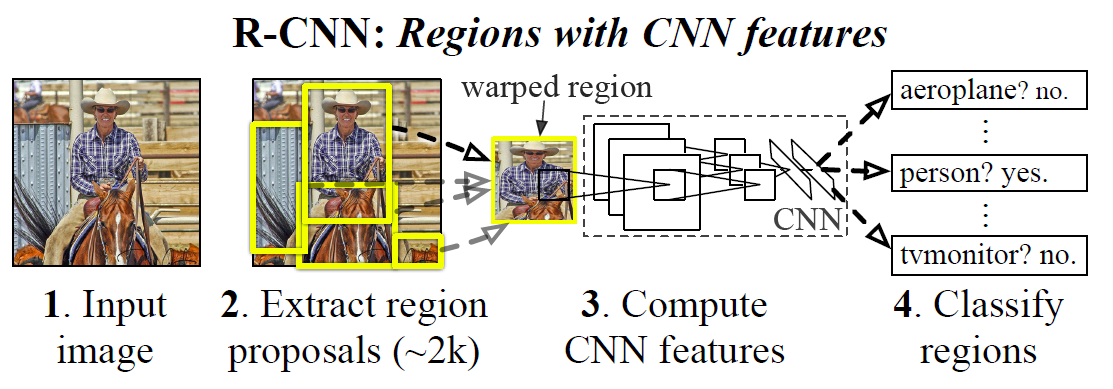
In 2013, Ross Girshick’s (abbreviated as RBG) R-CNN paper Rich feature… emerged, which is also the pioneering work in using convolutional neural networks for object detection.
R-CNN is short for Regions with CNN features, which means region-based convolutional neural network. Its main idea generally includes three steps:
-
Use the heuristic algorithm Selective search paper to generate approximately 2000 Region proposal regions to be detected.
-
Input each Region proposal into a convolutional neural network to extract features, and then use a support vector machine to complete classification.
-
Train a linear regression model to shrink the bounding box.
Next, we will introduce these three steps in detail.
Traditional region selection uses the idea of a sliding window. A sliding window means that after specifying a window, it moves sequentially on the image at equal intervals. In this way, each time the window slides, a detection is performed. The information of adjacent windows overlaps highly, resulting in a slow detection speed.
However, R-CNN uses the Selective search algorithm. It first generates candidate regions all at once and then performs detection. Although Selective search generates approximately 2000 Region proposals for each image, the number is much lower compared to the exhaustive sliding window search. Regarding the Selective search method, you can read the paper What makes…, which also compares other relevant candidate bounding box search algorithms in addition to Selective search.
Next, each Region proposal is input into a convolutional neural network to extract features, and then a support vector machine is used to complete the classification. In this process, the support vector machine solves a binary classification problem, that is, to judge whether it belongs to this category, either “yes” or “no”.
For a bounding box, we generally use the \((x, y, w, h)\) coordinates to represent its position. \((x, y)\) are the coordinates of the center point, \(w\) represents the width of the image, and \(h\) represents the height of the image.

Since the coordinates are numerical values, they can actually be regarded as a regression problem, and then the position of the bounding box can be corrected. R-CNN cited the relevant method proposed in the paper Object Detection….
Although R-CNN has much higher detection accuracy than traditional methods, there are still more than 2,000 candidate regions, which results in a very slow detection speed. Subsequently, researchers proposed different improvement methods, and the development sequence is: R-CNN → SPP Net → Fast R-CNN → Faster R-CNN → Mask R-CNN.
SPP Net paper was proposed by the team of He Kaiming, which mainly improved the generation of candidate regions and the convolution order, and broke the bondage of fixed-size input. Subsequently, RBG improved R-CNN and proposed Fast R-CNN paper. It cited the work of SPP Net and mainly optimized the workflow to improve efficiency.
Later, the team of He Kaiming and RBG joined hands again to propose Faster R-CNN paper, which means it can be made even faster. The main improvement of this method is to use a neural network to generate candidate regions instead of the previous selective search, thus further improving the accuracy of the bounding box. In 2017, the two joined hands again to release Mask R-CNN paper. This method can not only perform “object detection”, but also perform “semantic segmentation” at the same time, thus updating the R-CNN family once again.
68.3.2. YOLO and SSD#
We summarize the idea of the R-CNN family, which is actually roughly divided into two steps, that is, to generate Region Proposal first or to extract features using CNN first, and then use a classifier to classify and correct the position of the bounding box.
In 2015, the YOLO method was proposed paper. Different from the two-step strategy of the R-CNN family, YOLO directly uses a regression method to determine the bounding box in one step. How does it achieve this?
The full name of YOLO is You Only Look Once, that is, “You only need to look once”. Its solution is simple and straightforward, and it looks similar to the road condition detection system built at the beginning of the experiment. Here, we directly quote the pictures in the paper for explanation.
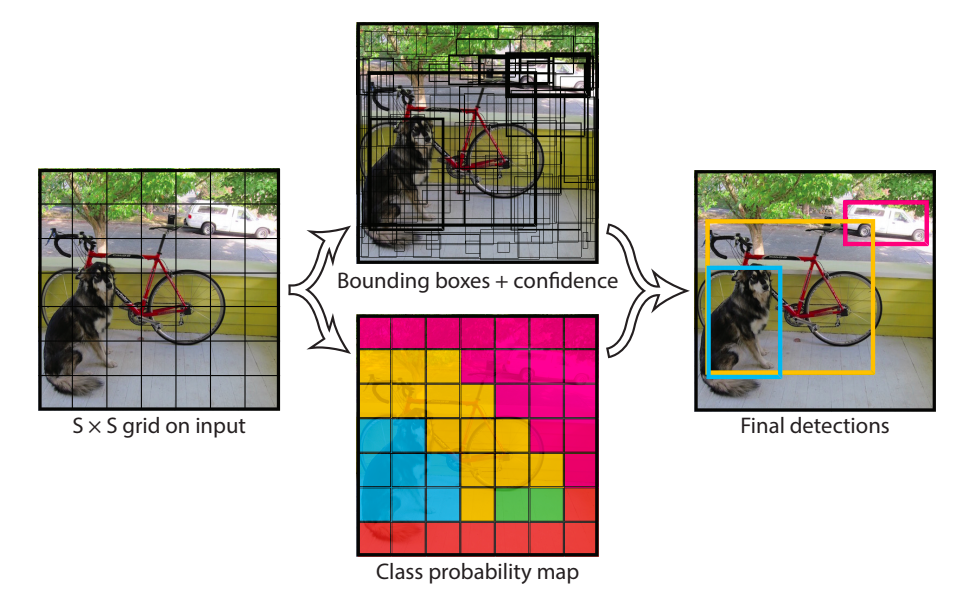
As shown in the figure above, the sample input image is divided into a \(7*7\) grid. Next, each grid is detected and the \((x, y, w, h)\) and confidence of the bounding box are output. Among them, the confidence includes the category of the object within the grid and the prediction accuracy. Finally, after processing each grid, the Non-Maximum Suppression (NMS) algorithm is used to remove overlapping boxes and obtain the result.
YOLO improved the detection speed, but it didn’t perform well on small objects. So SSD paper added the concept of Anchor in Faster R-CNN to YOLO and made predictions by integrating the features of different convolutional layers.
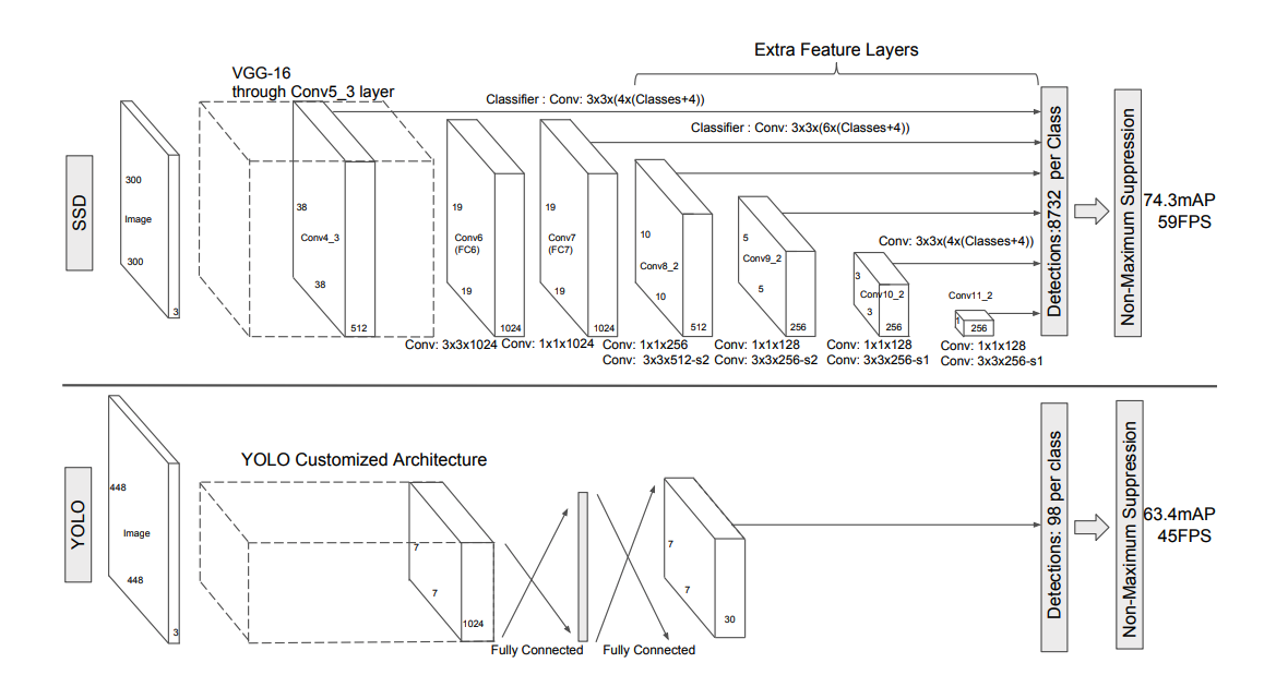
You can see the differences from the network structure above. SSD combines the features extracted from Feature Maps of different sizes and then makes predictions, improving the detection accuracy for small objects. In addition, SSD eliminates the fully connected layers, reduces the parameters, and improves the speed.
68.4. Object Detection Applications#
Above, we introduced the two main types of methods in the field of object detection. In fact, you can summarize them as one-step or two-step implementations. YOLO and SSD are typical one-step methods that directly utilize the excellent performance of the classifier to regress the bounding box positions. The R-CNN family is a two-step implementation that generally requires obtaining Region proposals first and then using classification to correct the bounding boxes. Of course, these two types of methods also have their own advantages. The main advantages of YOLO and SSD are “fast”, while the R-CNN family is more “accurate”.
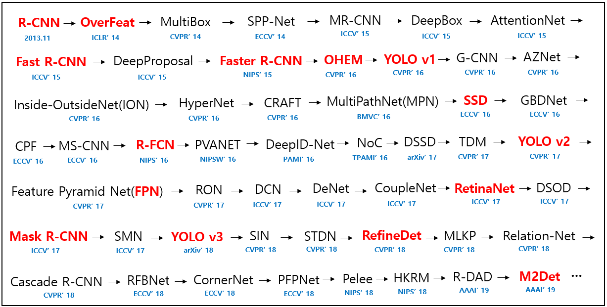
If you want to know the development roadmap of object detection in the academic field in recent years, you can follow the A paper list… project, which summarizes a relatively complete roadmap of method proposals.
Next, we will try how to truly apply object detection.
68.4.1. Mask R-CNN#
Mask R-CNN is one of the most excellent methods in the R-CNN family. Mask R-CNN can not only complete “object detection”, but also be used for “semantic segmentation” in computer vision at the same time. Next, we will try to use Mask R-CNN to complete the image object detection task.
Regarding the implementation of the Mask R-CNN model, we will not study it in this experiment because it involves too much extended professional knowledge and the model is relatively complex. Interested students can read the original paper and refer to the model implementation code.
Next, we will download the code related to the pre-implemented Mask R-CNN model and install the dependency libraries required for this experiment.
{note}
Mask R-CNN currently only supports TensorFlow 1.x, and the corresponding code cannot be executed on TensorFlow 2. Wait for updates and fixes.
# 安装过程可能需持续数分钟,请耐心等待执行完成
!git clone "https://github.com/huhuhang/Mask_RCNN.git"  # 克隆所需代码
pip install -r "Mask_RCNN/requirements.txt"  # 安装依赖库
Training Mask R-CNN from scratch is difficult because you need to manually label your own dataset. Therefore, in this experiment, we still adopt the idea of using a pre-trained model to experience the object detection process. First, here we introduce the COCO dataset.
You should be very familiar with the ImageNet dataset, which is a commonly used benchmark dataset for image classification. Most relevant research papers also cite the test results on this dataset to demonstrate the innovation and improvement of their own research. COCO is also a well-known benchmark dataset, which is often used in the fields of object detection, semantic segmentation, etc. This dataset was contributed by Microsoft and was first proposed in the paper Microsoft COCO….
COCO currently contains more than 330,000 images, most of which have been manually labeled, that is, the object bounding boxes have been manually defined. Although the COCO dataset only contains 80 object categories, the number of images in each category is large, so it can improve the detection ability of the model for specific categories. You can preview the dataset through the officially provided page.
Next, you need to import the custom Mask R-CNN related
libraries. Load them by specifying the path through
sys.path.append. The library name is
mrcnn.
import sys
import warnings
warnings.filterwarnings('ignore')
sys.path.append("Mask_RCNN")  # 链接到自定义 mrcnn 库
sys.path.append("Mask_RCNN/samples/coco/")  # 链接到自定义 COCO 模块
We download the pre-trained model [258 MB] of Mask R-CNN on the COCO dataset.
import os
from mrcnn import utils

# 下载 Mask R-CNN 在 COCO 数据集上的预训练模型
utils.download_trained_weights("mask_rcnn_coco.h5")
Then, we will use the model
mask_rcnn_coco.h5
trained on the COCO dataset. The configuration of this
model is in the
CocoConfig
class in
coco.py. Since the goal of the experiment is model inference
(object detection), we need to inherit from the
CocoConfig
class and modify the configuration attributes to adapt to
the inference process.
import coco

class InferenceConfig(coco.CocoConfig):
    # 设置 Batch size = 1 方便在单张图片上推理
    # Batch size = GPU_COUNT * IMAGES_PER_GPU
    GPU_COUNT = 1
    IMAGES_PER_GPU = 1

config = InferenceConfig()
config.display()
Next, use
mrcnn.model.MaskRCNN
to initialize the model and set it to inference mode, and
at the same time import the pre-trained model weights.
import mrcnn.model as modellib

MODEL_DIR = os.path.abspath("logs")  # 存放训练模型及日志路径
# 新建模型并置于推理模式
model = modellib.MaskRCNN(mode="inference", model_dir=MODEL_DIR, config=config)
# 加载预训练模型权重
model.load_weights("mask_rcnn_coco.h5", by_name=True)
model
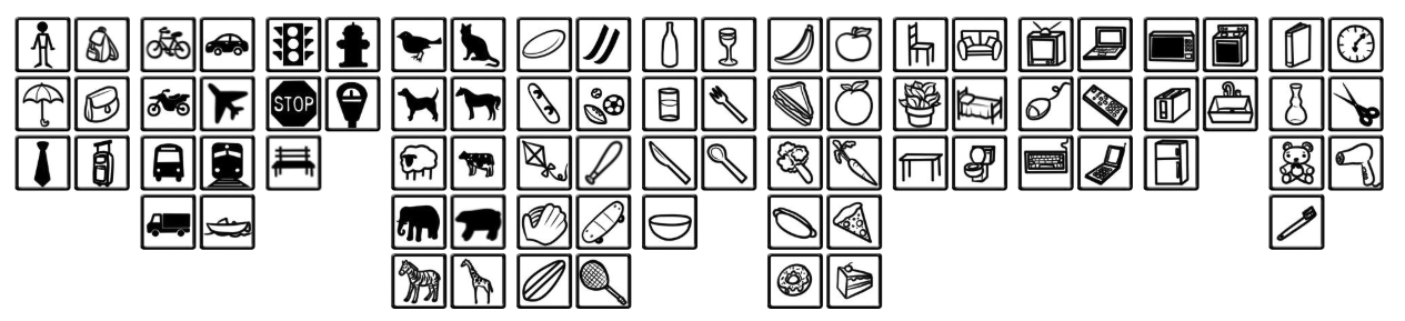
As introduced above, the COCO dataset has achieved the calibration of 80 commonly used object categories. For the labels of these categories, you can import them through the following code.
import coco

dataset = coco.CocoDataset() # Download the COCO dataset
dataset.load_coco(COCO_DIR, "train")
dataset.prepare()
print(dataset.class_names) # Print the categories
Since the COCO dataset is too large, about 18 GB, it will not be directly downloaded here. The experiment will manually define the labels of object categories according to the encoding order of labels in COCO.
# COCO 类别名称,顺序相关
class_names = ['BG', 'person', 'bicycle', 'car', 'motorcycle', 'airplane',
               'bus', 'train', 'truck', 'boat', 'traffic light',
               'fire hydrant', 'stop sign', 'parking meter', 'bench', 'bird',
               'cat', 'dog', 'horse', 'sheep', 'cow', 'elephant', 'bear',
               'zebra', 'giraffe', 'backpack', 'umbrella', 'handbag', 'tie',
               'suitcase', 'frisbee', 'skis', 'snowboard', 'sports ball',
               'kite', 'baseball bat', 'baseball glove', 'skateboard',
               'surfboard', 'tennis racket', 'bottle', 'wine glass', 'cup',
               'fork', 'knife', 'spoon', 'bowl', 'banana', 'apple',
               'sandwich', 'orange', 'broccoli', 'carrot', 'hot dog', 'pizza',
               'donut', 'cake', 'chair', 'couch', 'potted plant', 'bed',
               'dining table', 'toilet', 'tv', 'laptop', 'mouse', 'remote',
               'keyboard', 'cell phone', 'microwave', 'oven', 'toaster',
               'sink', 'refrigerator', 'book', 'clock', 'vase', 'scissors',
               'teddy bear', 'hair drier', 'toothbrush']
The first in
class_names
is the background, and the subsequent ones are the labels
of 80 object categories. Since it is related to the
calibration order during training, this label order cannot
be modified, otherwise the final calibrated categories
will be confused.
Finally, we select the example image at the beginning of the experiment for object detection.
import requests
from skimage import io
from matplotlib import pyplot as plt
%matplotlib inline

# 下载图片并保存为 test.jpg
url = "https://cdn.aibydoing.com/aibydoing/images/document-uid214893labid7506timestamp1551679627073.jpg"
with open("test.jpg", "wb") as f:
    f.write(requests.get(url).content)

plt.imshow(io.imread("test.jpg"))
model.detect
can be used for object detection and finally returns
coordinate information such as bounding boxes. Then, the
calibration is visualized through
mrcnn.visualize.
from mrcnn import visualize

image = io.imread("test.jpg")
results = model.detect([image], verbose=1)  # 运行检测
r = results[0]  # 可视化结果
visualize.display_instances(image, r['rois'], r['masks'],
                            r['class_ids'], class_names, r['scores'])
It can be seen that most of the calibrations are fine and
the bounding boxes are relatively accurate. However, the
radar of the autonomous vehicle shown in the middle of the
bottom of the image is marked as
person, which should be an obvious error.
So far, we have completed the process of inference using the pre-trained model of Mask R-CNN on COCO. The whole process is relatively simple. For the 80 categories of objects covered by the COCO dataset, the model can be used without any modification. However, if you want to calibrate specific objects in your own provided dataset, you need to manually create the dataset and start the training of Mask R-CNN again. Here is an article Instance Segmentation… for your reference.
68.4.2. TensorFlow Object Detection#
In fact, TensorFlow also provides a set of object detection tools called TensorFlow Object Detection API, which is currently part of the TensorFlow Research program. The TensorFlow Object Detection API provides more than a dozen pre-trained models, and you can learn about them in detail through the official documentation page. Each set of models provides the selected usage method and training dataset, and also indicates the performance.
Model name |
Speed (ms) |
COCO mAP |
Outputs |
|---|---|---|---|
|
ssd_mobilenet_v1_coco |
30 |
21 |
Boxes |
|
ssd_mobilenet_v1_0.75_depth_coco |
26 |
18 |
Boxes |
|
ssd_mobilenet_v1_quantized_coco |
29 |
18 |
Boxes |
|
ssd_mobilenet_v1_0.75_depth_quantized_coco |
29 |
16 |
Boxes |
…… |
…… |
…… |
…… |
Similarly, next we refer to the example provided by the official to try to use the TensorFlow Object Detection API to complete model inference. First, you need to clone the source code related to TensorFlow Object Detection, and the source code has been appropriately optimized for this experiment.
!git clone "https://github.com/huhuhang/object_detection.git"  # 克隆所需代码
sys.path.append("object_detection")  # 链接到自定义 mrcnn 库
In addition, since the TensorFlow Object Detection API uses Protobufs to configure the model and training parameters, the Protobuf library must be compiled before using the framework.
!apt-get update
!apt-get install --yes protobuf-compiler # 安装编译工具
!protoc object_detection/protos/*.proto --python_out=.
First, download a pre-trained model provided by TensorFlow. Here, select the model that uses SSD to complete training on the COCO dataset and uses Mobilenet for feature extraction. The reason for choosing this model is that it is relatively small in size, but the effect is not the best. For more pre-trained models, you can find the download links provided by TensorFlow through this page.
import six.moves.urllib as urllib
import tarfile

# 定义下载路径
MODEL_NAME = 'ssd_mobilenet_v1_coco_2017_11_17'
MODEL_FILE = MODEL_NAME + '.tar.gz'
DOWNLOAD_BASE = 'http://download.tensorflow.org/models/object_detection/'
PATH_TO_FROZEN_GRAPH = MODEL_NAME + '/frozen_inference_graph.pb'

# 下载预训练模型并解压
opener = urllib.request.URLopener()
opener.retrieve(DOWNLOAD_BASE + MODEL_FILE, MODEL_FILE)
tar_file = tarfile.open(MODEL_FILE)
for file in tar_file.getmembers():
    file_name = os.path.basename(file.name)
    if 'frozen_inference_graph.pb' in file_name:
        tar_file.extract(file, os.getcwd())
        print("下载并解压完成.")
The model has been downloaded to the path
ssd_mobilenet_v1_coco_2017_11_17/frozen_inference_graph.pb. Next, we need to load the pre-trained model into
memory.
import tensorflow as tf

detection_graph = tf.Graph()
with detection_graph.as_default():
    od_graph_def = tf.GraphDef()
    with tf.gfile.GFile(PATH_TO_FROZEN_GRAPH, 'rb') as fid:
        serialized_graph = fid.read()
        od_graph_def.ParseFromString(serialized_graph)
        tf.import_graph_def(od_graph_def, name='')
At this point, a function
run_inference_for_single_image
needs to be defined to perform inference detection on a
single image using the model. This function is taken from
the source code and is relatively complex and can be
executed directly.
import numpy as np
from object_detection.utils import ops as utils_ops

def run_inference_for_single_image(image, graph):
    with graph.as_default():
        with tf.Session() as sess:
            # Get handles to input and output tensors
            ops = tf.get_default_graph().get_operations()
            all_tensor_names = {
                output.name for op in ops for output in op.outputs}
            tensor_dict = {}
            for key in [
                'num_detections', 'detection_boxes', 'detection_scores',
                'detection_classes', 'detection_masks'
            ]:
                tensor_name = key + ':0'
                if tensor_name in all_tensor_names:
                    tensor_dict[key] = tf.get_default_graph().get_tensor_by_name(
                        tensor_name)
            if 'detection_masks' in tensor_dict:
                # The following processing is only for single image
                detection_boxes = tf.squeeze(
                    tensor_dict['detection_boxes'], [0])
                detection_masks = tf.squeeze(
                    tensor_dict['detection_masks'], [0])
                real_num_detection = tf.cast(
                    tensor_dict['num_detections'][0], tf.int32)
                detection_boxes = tf.slice(detection_boxes, [0, 0], [
                                           real_num_detection, -1])
                detection_masks = tf.slice(detection_masks, [0, 0, 0], [
                                           real_num_detection, -1, -1])
                detection_masks_reframed = utils_ops.reframe_box_masks_to_image_masks(
                    detection_masks, detection_boxes, image.shape[0], image.shape[1])
                detection_masks_reframed = tf.cast(
                    tf.greater(detection_masks_reframed, 0.5), tf.uint8)
                # Follow the convention by adding back the batch dimension
                tensor_dict['detection_masks'] = tf.expand_dims(
                    detection_masks_reframed, 0)
            image_tensor = tf.get_default_graph().get_tensor_by_name('image_tensor:0')

            # Run inference
            output_dict = sess.run(tensor_dict,
                                   feed_dict={image_tensor: np.expand_dims(image, 0)})

            # all outputs are float32 numpy arrays, so convert types as appropriate
            output_dict['num_detections'] = int(
                output_dict['num_detections'][0])
            output_dict['detection_classes'] = output_dict[
                'detection_classes'][0].astype(np.uint8)
            output_dict['detection_boxes'] = output_dict['detection_boxes'][0]
            output_dict['detection_scores'] = output_dict['detection_scores'][0]
            if 'detection_masks' in output_dict:
                output_dict['detection_masks'] = output_dict['detection_masks'][0]
    return output_dict
Finally, read the test image, perform object detection, and complete the visualization of the bounding boxes.
from utils import visualization_utils as vis_util
from utils import label_map_util

# 读取测试图片
image_np = io.imread("test.jpg")
# 图片数组处理成模型期望的形状 [1, None, None, 3]
image_np_expanded = np.expand_dims(image_np, axis=0)
# COCO 数据集标签
PATH_TO_LABELS = os.path.join('object_detection/data', 'mscoco_label_map.pbtxt')
category_index = label_map_util.create_category_index_from_labelmap(
    PATH_TO_LABELS, use_display_name=True)
# 目标检测
output_dict = run_inference_for_single_image(image_np, detection_graph)
# 可视化检测边界框
vis_util.visualize_boxes_and_labels_on_image_array(
    image_np,
    output_dict['detection_boxes'],
    output_dict['detection_classes'],
    output_dict['detection_scores'],
    category_index,
    instance_masks=output_dict.get('detection_masks'),
    use_normalized_coordinates=True,
    line_thickness=10)
plt.figure(figsize=(12, 8))
plt.imshow(image_np)
As you can see, compared with the previous experiment using the Mask R-CNN pre-trained model, the SSD MobileNet is much less impressive. Traffic lights, pedestrians, etc. were not successfully detected. Of course, after all, the pre-trained model of the latter is only 1/10 the size of the former and is usually deployed on mobile platforms.
68.5. Summary#
In this experiment, we learned about the history and development of object detection technology in computer vision and got to know various object detection methods based on deep learning techniques. Among them, we focused on learning about the R-CNN family and used the pre-trained model provided by MASK R-CNN to complete the detection and inference process for common object categories. Subsequently, the experiment introduced TensorFlow Object Detection and completed a simple process example. If you are interested in the field of object detection, you still need to continue learning how to train on custom datasets.
Related Links