
66. Autoencoder Principle and Construction#
66.1. Introduction#
Previously, we learned about the Generative Adversarial Network (GAN). You should be able to notice that if we classify it according to supervised learning and unsupervised learning, GAN is obviously an unsupervised learning neural network because we don’t need to label the data. In this experiment, the autoencoder that we are about to come into contact with is also an unsupervised neural network. This experiment will help you understand its principle and function.
66.2. Key Points#
Introduction to Autoencoders
Basic Autoencoders
Denoising Autoencoders
66.3. Introduction to Autoencoders#
An autoencoder, also known as a self - encoder, is an artificial neural network used in the process of unsupervised learning. An autoencoder usually consists of two parts: an encoder and a decoder. Below, we will explain it through a diagram.
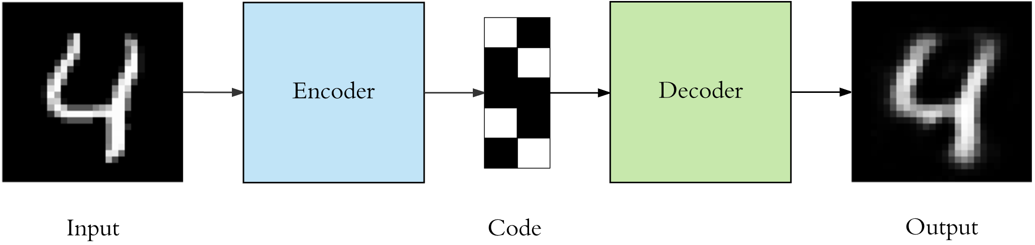
The above figure shows the classic process of an autoencoder: The input is encoded into a Code by the Encoder neural network and then output after being processed by the Decoder neural network. Among them:
-
Encoder: Compresses the input into a latent space representation.
-
Decoder: Reconstructs and decodes the latent space representation.
You may notice that after the handwritten character 4 in the above figure is processed by the autoencoder, it still looks like the handwritten character 4. So what exactly is the use of the autoencoder?
If the purpose of the autoencoder is to repeat the input and output features, it would surely be useless. In fact, we hope to make the latent representation have valuable properties by training an autoencoder with the output value equal to the input value. At the same time, the autoencoder completes the reconstruction of the input features. Therefore, the autoencoder also has two main uses: data denoising and dimensionality reduction for data visualization.
66.4. Basic Autoencoder#
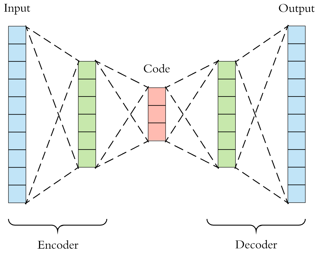
Before formally constructing the autoencoder, we need to further understand the characteristics of the autoencoder network. First, both the encoder and decoder in the autoencoder are fully connected feedforward neural network structures as shown below. You can freely define the hyperparameters of the two neural networks, and of course, they are not necessarily symmetric structures as shown below.
For the convenience of demonstration, the familiar MNIST dataset is used in the experiment.
Next, we first use Keras to load this dataset. At the same time, the handwritten character images are flattened and normalized by dividing by 255. To improve the training speed, only 30,000 training samples and 100 test samples are selected for the experiment.
import tensorflow as tf

(X_train, _), (X_test, _) = tf.keras.datasets.mnist.load_data()
X_train = X_train[:30000].reshape(-1, 28 * 28) / 255
X_test = X_test[:100].reshape(-1, 28 * 28) / 255

X_train.shape, X_test.shape
Downloading data from https://storage.googleapis.com/tensorflow/tf-keras-datasets/mnist.npz
11490434/11490434 [==============================] - 2s 0us/step
((30000, 784), (100, 784))
Next, we build a very simple basic autoencoder structure that only contains 1 hidden layer. To make it easier to clarify the encoder and decoder parts, instead of using the Keras sequential model in this experiment, we use the functional API to build it.
# 输出
input_ = tf.keras.layers.Input(shape=(784,))
# 编码器
encoded = tf.keras.layers.Dense(64, activation="relu")(input_)
# 解码器
decoded = tf.keras.layers.Dense(784, activation="sigmoid")(encoded)

# 建立函数模型,传入输入和输出层
model = tf.keras.models.Model(inputs=input_, outputs=decoded)
model.summary()
Model: "model"
_________________________________________________________________
 Layer (type)                Output Shape              Param #
=================================================================
 input_1 (InputLayer)        [(None, 784)]             0

 dense (Dense)               (None, 64)                50240

 dense_1 (Dense)             (None, 784)               50960

=================================================================
Total params: 101200 (395.31 KB)
Trainable params: 101200 (395.31 KB)
Non-trainable params: 0 (0.00 Byte)
_________________________________________________________________
In the classic autoencoder structure, generally, the output layer of the encoder uses the ReLU activation, while the output layer of the decoder uses the Sigmoid activation. Therefore, we also follow this structure above.
Next, we try to compile the model. Among them, the familiar
Adam optimizer can be selected, and the loss function
generally chooses cross-entropy or mean squared error (MSE).
From an empirical perspective, if the input values are in
the range of
\([0, 1]\), the cross-entropy loss function
binary_crossentropy
is usually used; otherwise, the mean squared error is used.
The input values of the MNIST dataset are originally between
\([0, 255]\). Since we have completed the normalization operation, the
cross-entropy loss function is selected.
model.compile(optimizer="adam", loss="binary_crossentropy")
Finally, it comes to the training process of the autoencoder. It should be noted that the target of the autoencoder is the same as the input, so in Keras, the label parameter can be passed in with the features.
model.fit(X_train, X_train, batch_size=64, epochs=10)
Epoch 1/10
469/469 [==============================] - 1s 1ms/step - loss: 0.2034
Epoch 2/10
469/469 [==============================] - 1s 1ms/step - loss: 0.1229
Epoch 3/10
469/469 [==============================] - 1s 1ms/step - loss: 0.1013
Epoch 4/10
469/469 [==============================] - 1s 2ms/step - loss: 0.0900
Epoch 5/10
469/469 [==============================] - 1s 1ms/step - loss: 0.0836
Epoch 6/10
469/469 [==============================] - 1s 1ms/step - loss: 0.0801
Epoch 7/10
469/469 [==============================] - 1s 1ms/step - loss: 0.0780
Epoch 8/10
469/469 [==============================] - 1s 1ms/step - loss: 0.0767
Epoch 9/10
469/469 [==============================] - 1s 1ms/step - loss: 0.0758
Epoch 10/10
469/469 [==============================] - 1s 1ms/step - loss: 0.0752
<keras.src.callbacks.History at 0x2968ba380>
Next, we do two things, namely: visualize the Code after the test data passes through the encoder, and visualize the output image after reconstruction by the decoder.
First, to view the output of the encoder, we need to define the encoder model and then perform inference.
from matplotlib import pyplot as plt

%matplotlib inline

n = 5
encoder = tf.keras.models.Model(input_, encoded)  # 仅编码器模型
encoded_code = encoder.predict(X_test[:n])  # 编码器之后的 Code
# 可视化前 10 个测试样本编码之后的 Code
plt.figure(figsize=(10, 8))
for i in range(n):
    ax = plt.subplot(1, n, i + 1)
    plt.imshow(encoded_code[i].reshape(4, 16).T, cmap="gray")
    ax.get_xaxis().set_visible(False)  # 不显示坐标
    ax.get_yaxis().set_visible(False)
1/1 [==============================] - 0s 29ms/step

The Code after some test data is processed by the trained encoder is shown above. Of course, it looks like a mess of characters.
However, next, we use the complete autoencoder including the decoder to reconstruct the test data. Then, compare the test samples with the images of the test samples output by the autoencoder.
decoded_code = model.predict(X_test[:n])  # 自动编码器推理
plt.figure(figsize=(10, 6))
for i in range(n):
    # 输出原始测试样本图像
    ax = plt.subplot(3, n, i + 1)
    plt.imshow(X_test[i].reshape(28, 28), cmap="gray")
    ax.get_xaxis().set_visible(False)
    ax.get_yaxis().set_visible(False)

    # 输出自动编码器重构后的图像
    ax = plt.subplot(3, n, i + n + 1)
    plt.imshow(decoded_code[i].reshape(28, 28), cmap="gray")
    ax.get_xaxis().set_visible(False)
    ax.get_yaxis().set_visible(False)
1/1 [==============================] - 0s 17ms/step

You will find that the output structure after reconstruction by the decoder is very similar to the original result. So what does this indicate?
Actually, the previous steps demonstrated the process of using an autoencoder to perform dimensionality reduction (compression) on data. The encoder encodes the original sample of length 784 into a Code of length 64, which is the process of compressing the input into a latent space representation. And the decoder actually reconstructs an image very close to the original sample from the Code of length 64. So, can we use the compressed features to replace the original sample features? The answer is definitely yes.
66.5. Denoising Autoencoder#
Above, we built a basic autoencoder and learned about the application of autoencoders in data dimensionality reduction. Next, the experiment will take you to learn another classic scenario of autoencoders: data denoising.
First, we add random Gaussian noise to the above MNIST
dataset. The idea is simple. First, use
np.random.normal
to generate random values of the same size and add them to
the original array. Then use
np.clip
to normalize the array to the range
\([0, 1]\).
The following process may take a while. Please be patient.
import numpy as np

X_train_ = X_train + 0.4 * np.random.normal(size=X_train.shape)  # 添加同尺寸随机值
X_test_ = X_test + 0.4 * np.random.normal(size=X_test.shape)
X_train_noisy = np.clip(X_train_, 0, 1)  # 将数组规约到 [0, 1] 之间
X_test_noisy = np.clip(X_test_, 0, 1)

X_train_noisy.shape, X_test_noisy.shape
((30000, 784), (100, 784))
Next, we visualize the sample images after adding random noise.
plt.figure(figsize=(10, 2))
for i in range(n):
    ax = plt.subplot(1, n, i + 1)
    plt.imshow(X_train_noisy[i].reshape(28, 28), cmap="gray")
    ax.get_xaxis().set_visible(False)
    ax.get_yaxis().set_visible(False)

Next, we hope that the autoencoder can regenerate the original image based on the noisy image. The process is shown in the following figure.
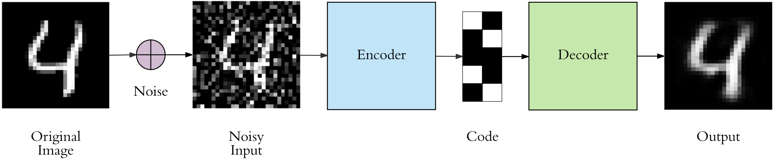
You can modify the above basic autoencoder to make it more complex. Of course, you can also continue to use the basic autoencoder structure defined above. Slightly different is that the input during training is the noisy image, while the target value is the original image.
model.fit(X_train_noisy, X_train, batch_size=64, epochs=10)
Epoch 1/10
469/469 [==============================] - 1s 1ms/step - loss: 0.1071
Epoch 2/10
469/469 [==============================] - 1s 1ms/step - loss: 0.1015
Epoch 3/10
469/469 [==============================] - 1s 2ms/step - loss: 0.1003
Epoch 4/10
469/469 [==============================] - 1s 2ms/step - loss: 0.0997
Epoch 5/10
469/469 [==============================] - 1s 2ms/step - loss: 0.0994
Epoch 6/10
469/469 [==============================] - 1s 2ms/step - loss: 0.0991
Epoch 7/10
469/469 [==============================] - 1s 2ms/step - loss: 0.0989
Epoch 8/10
469/469 [==============================] - 1s 1ms/step - loss: 0.0988
Epoch 9/10
469/469 [==============================] - 1s 1ms/step - loss: 0.0986
Epoch 10/10
469/469 [==============================] - 1s 1ms/step - loss: 0.0985
<keras.src.callbacks.History at 0x29ec05180>
Next, use the noisy image data in the test data for the experiment and see if the noise can be successfully removed after being processed by the trained autoencoder.
decoded_code = model.predict(X_test_noisy[:n])  # 自动编码器推理
plt.figure(figsize=(10, 6))
for i in range(n):
    # 输出原始测试样本图像
    ax = plt.subplot(3, n, i + 1)
    plt.imshow(X_test_noisy[i].reshape(28, 28), cmap="gray")
    ax.get_xaxis().set_visible(False)
    ax.get_yaxis().set_visible(False)

    # 输出自动编码器去噪后的图像
    ax = plt.subplot(3, n, i + n + 1)
    plt.imshow(decoded_code[i].reshape(28, 28), cmap="gray")
    ax.get_xaxis().set_visible(False)
    ax.get_yaxis().set_visible(False)
1/1 [==============================] - 0s 11ms/step

As can be seen, the results are quite good. The autoencoder after training has successfully removed most of the noise in the test data. Of course, the network used here is still relatively basic. If a convolutional autoencoder structure is used, the effect will be better.
66.6. Summary#
In this experiment, we learned what an autoencoder is and how to build an autoencoder. Of course, the experiment also completed the process of dimensionality reduction and denoising of MNIST data through a basic autoencoder structure. Autoencoders are currently developing well, especially the more advanced and complex Variational Autoencoder. Students who are interested can also learn about it by themselves.