64. Principle and Construction of Generative Adversarial Networks#
64.1. Introduction#
In this section of the experiment, we will officially start learning about Generative Adversarial Nets (GAN). Yann LeCun, the main person in charge of Facebook AI, once clearly stated that generative adversarial networks are the most interesting idea in the field of machine learning in the past decade. It has to be said that generative adversarial networks have become the representative of the currently hottest unsupervised deep learning and are constantly developing new applications in the entire industrial community.
64.2. Key Points#
Principle of Generative Adversarial Networks
-
Implementation of Generative Adversarial Networks
-
Improvement of Generative Adversarial Networks
Future of Generative Adversarial Networks
64.3. Principle of Generative Adversarial Networks#
Generative Adversarial Networks (https://arxiv.org/abs/1406.2661v1) is an unsupervised learning method proposed by Ian Goodfellow et al. in 2014. The characteristic of this method is to learn by having two neural networks play against each other. GAN has advantages in image generation, especially the later derivatives such as DCGAN, BiGAN, BigGAN, etc.
Before formally introducing Generative Adversarial Networks, let’s first take a look at an interesting conversation:
Male painter: Hey, do you think my painting looks good? Girlfriend: What the heck is this? Can’t you make the proportions more symmetrical? Male painter: Oh, then I’ll go and fix it.
Male painter: How about this one? I’ve made the proportions symmetrical. Girlfriend: Oh, come on. Please go and learn how to color properly. Male painter: Oh, then I’ll go and fix it.
Male painter: Is it better this time? I’ve colored it evenly. Girlfriend: Oh, come on. Put your painting next to Master Van Gogh’s, and you can immediately see the difference.
Male painter: How about this one? I’ve practiced a lot. Girlfriend: Well, then I’ll have it framed and claim it’s an authentic work by Master Van Gogh.
This is the growth process of a male painter under the ultimate decision-making criterion of his girlfriend, based on the works of Master Van Gogh. In fact, generative adversarial networks are built according to this principle. Now let’s take a detailed look.
As shown in the figure below, the male painter is equivalent to the generator, which can generate a painting from a pile of pigments and lines (the output of the generator, which is also a fake). His girlfriend acts as the discriminator here, comparing the real data, that is, the works of Master Van Gogh, with it for discrimination.
During the entire training process of the male painter, the male painter’s goal is to make his girlfriend think that his works are indistinguishable from those of Master Van Gogh. And in order to train him, his girlfriend tries to pick out the differences between his works and those of Master Van Gogh as if she were being picky. Eventually, the male painter’s works can achieve the goal of passing off as genuine, and then he has fully grown. During this process, the generator and the discriminator are always in an adversarial state, which is the origin of the name of the generative adversarial network.
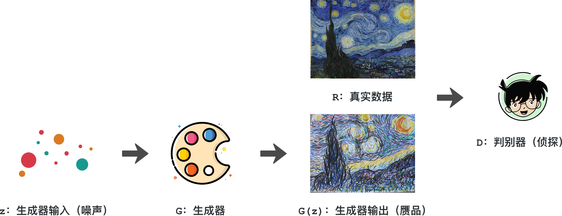
Now, let’s replace the whole scenario with a neural network. First, by inputting a distribution of data into the generator, the generator learns to generate an output (a fake) through the neural network, and this output is input into the discriminator together with the real data. Then, the discriminator learns to distinguish the differences between the two through the neural network and makes a classification judgment on whether this work is genuine or fake.
In this way, the generator keeps training to pass off as genuine, and the discriminator keeps training to distinguish between the two. Eventually, the generator can truly simulate an output that is exactly the same as the real data, and the discriminator is no longer able to make a judgment. Based on Ian Goodfellow’s earliest definition of GAN, GAN is actually completing such a mathematical optimization task:
In the formula, \(G\) represents the generator, \(D\) represents the discriminator, \(V\) is the defined value function, representing the discrimination performance of the discriminator, and the larger this value, the better the performance. \(p_{data}(x)\) represents the real data distribution, \(p_{z}(z)\) represents the input data distribution of the generator, and \(E\) represents the expectation.
Note
The following part of the formula interpretation requires a certain mathematical theory foundation. You can skip it if you can’t understand.
The first term \(E_{p_{data}}\left ( x \right )[\log D(x)]\) is constructed based on the logarithmic function loss of real data. Specifically, it can be understood that in the most ideal situation, the discriminator \(D\) can give a judgment of 1 for the distribution data based on real data. Therefore, maximizing this term by optimizing \(D\) can make \(D(x) = 1\). Among them, \(x\) follows the \(p_{data}(x)\) distribution.
The second term, \(E_{p_{z}}\left ( z \right ) [\log (1 - D(G(z))]\), is for the generated data of the generator. We hope that when the data fed to the discriminator is the generated data of the generator, the discriminator can output 0. Since the output of \(D\) is the probability that the input data is real data, then \(1 - D(input)\) is the probability that the input data is the generated data of the generator. By optimizing \(D\) to maximize this term, we can make \(D(G(z)) = 0\). Among them, \(z\) follows \(p_{z}\), which is the generated data distribution of the generator.
So for the generator, what should we optimize?
The generator and the discriminator are in an adversarial relationship, and the value function represents the discrimination performance of the discriminator. Then, by optimizing \(G\), it can deceive the discriminator in the second term \(E_{p_{z}}\left ( z \right ) [\log (1 - D(G(z))]\), making the discriminator get \(D(G(z)) = 1\) as much as possible for the input \(G(z)\). Essentially, the generator is minimizing this term, that is, minimizing the value function.
So how to define the difference between two data distributions, that is, the real data and the data generated by the generator? Here, the concept of KL divergence needs to be introduced.
First, it can be proved that the KL divergence is non - negative. At the same time, it can also be found that when and only when \(P\) and \(Q\) are the same distribution for discrete variables, that is, \(p(x)=q(x)\), \(D_{KL}(P||Q)=0\). The KL divergence measures the degree of difference between two distributions and is often regarded as the distance between the two distributions.
However, it should be noted that \(D_{KL}(P||Q)\neq D_{KL}(Q||P)\), that is, the KL divergence does not have symmetry.
Next, fix the generator in the value function and write the expectation in integral form as:
In the whole expression, there is only one variable \(D\). Next, for the integrand, let \(y = D(x)\), \(a = p_{data}(x)\), \(b = p_{g}(x)\), where both \(a\) and \(b\) are constants. Then, the integrand becomes:
To find the optimal value of \(y\), the first derivative of the above equation needs to be taken. Moreover, when \(a + b\neq 0\), we have:
Verify that the second derivative \(f''(y)<0\) of \(f(y)\). Then the point \(\frac{a}{a + b}\) is a maximum value, and this fact gives the possibility of the existence of an optimal discriminator.
In fact, since in practice we do not know \(a = p_{data}(x)\), that is, the distribution of the real data. Then, in fact, we never use this formula to solve for our optimal discriminability. However, in fact, when we use deep learning to train the discriminator, we are making \(D\) gradually approach this goal.
If the optimal discriminator is as follows:
We substitute it into \(V(G,D)\), and at this time there is only one variable \(G\) in the value function:
At this time, through a rather skillful transformation, we can obtain the following expression:
This transformation is relatively complex. You can check the identity judgment between steps. According to some basic transformations of logarithms, we can obtain:
Finally, we get:
Due to the non-negativity of the KL divergence, it can be known that \(-\log4\) is the minimum value of \(V(G)\), and the minimum value is achieved if and only if \(p_{data}(x)=p_{g}(x)\). This actually means that the true data distribution is equal to the generated data distribution of the generator, and its existence and uniqueness can be proven theoretically from a mathematical perspective.
64.4. Generative Adversarial Network Implementation#
In the above section, we clarified what function GAN is optimizing and what purpose it is achieving. However, based solely on the above theoretical proof, there will be some problems in practice that need to be improved before it can be put into the actual practice process.
Input of the generator: That is, \(p_{z}(z)\) above. Of course, we cannot make this distribution arbitrary. Generally, it is set to common distribution types such as Gaussian distribution, uniform distribution, etc. Then the generator generates its own fake data based on the data generated from this distribution to deceive the discriminator.
How to simulate the expectation: In practice, we have no way to use integration to calculate the mathematical expectation. Therefore, generally, we can only sample from an infinite amount of real data and an infinite number of generators to approximate the true mathematical expectation.
Approximate value function: Given a generator \(G\) and wishing to compute \(maxV(G,D)\) to obtain the discriminator \(D\). Then, first, \(m\) samples \(\{x^{1}, x^{2}, \dots, x^{m}\}\) need to be sampled from the true data distribution \(p_{data}(x)\). And \(m\) samples \(\{\tilde{x}^{1}, \tilde{x}^{2}, \dots, \tilde{x}^{m}\}\) need to be sampled from the input of the generator, i.e., \(p_{z}(z)\). Thus, maximizing the value function \(V(G,D)\) can be approximately replaced using the following expression:
Therefore, the training process of GAN can be summarized as:
-
Sample \(m\) samples \(\{x^{1},x^{2}...,x^{m}\}\) from the real data \(p_{data}(x)\).
-
Sample \(m\) samples \(\{\tilde{x}^{1},\tilde{x}^{2},...,\tilde{x}^{m}\}\) from the input of the generator, i.e., the noise data \(p_{z}(z)\).
-
Feed the noise samples \(\{\tilde{x}^{1}, \tilde{x}^{2},..., \tilde{x}^{m}\}\) into the generator to generate \(\{G(\tilde{x}^{1}),G(\tilde{x}^{2}),...,G(\tilde{x}^{m})\}\).
-
Maximize the value function by gradient ascent to update the parameters of the discriminator.
-
Sample another \(m\) samples \(\{z^{1},z^{2},...,z^{m}\}\) from the input of the generator, i.e., the noise data \(p_{z}(z)\).
-
Feed the noise samples \(\{z^{1},z^{2},...,z^{m}\}\) into the generator to generate \(\{G(z^{1}),G(z^{2}),...,G(z^{m})\}\).
-
Minimize the value function by gradient descent to update the parameters of the generator.
At this point, you should have a preliminary impression of the training process of GAN. Next, let’s use code to deepen our understanding, and you will find that such training is very interesting.
First, import the modules we need. Here, we build a GAN based on PyTorch and complete the process of generating data for a handwritten recognition network. Among them, the real data will utilize the MNIST dataset in PyTorch.
import torch
from torchvision import datasets, transforms

transform = transforms.Compose([
    transforms.ToTensor(),
    transforms.Normalize(mean=[0.5], std=[0.5])
])

train_dataset = datasets.MNIST(root='.', train=True, download=True, transform=transform)
# 依旧采用 Mini-Batch 的训练方法,batch_size=128
dataloader = torch.utils.data.DataLoader(train_dataset, batch_size=64, shuffle=True)
dataloader
<torch.utils.data.dataloader.DataLoader at 0x1191f8280>
The
transform
function allows us to change the structure of the imported
dataset according to certain rules. Here, we introduce
Normalize
which will normalize the
Tensor. That is:
Normalized_image=(image
                      -
                      mean)/std
. The purpose of doing this is to facilitate subsequent
training. The code finally generates a training data loader.
Data preparation is complete. Next, let’s try to build a
deep learning model for constructing the discriminator and
the generator. Here, we build it by introducing the method
of the base class
nn.Module, which should be familiar after learning the previous
courses.
import torch.nn as nn


class Discriminator(nn.Module):
    # 判别器网络构建
    def __init__(self):
        super().__init__()
        self.model = nn.Sequential(
            nn.Linear(784, 1024),
            nn.ReLU(),
            nn.Dropout(0.3),
            nn.Linear(1024, 512),
            nn.ReLU(),
            nn.Dropout(0.3),
            nn.Linear(512, 256),
            nn.ReLU(),
            nn.Dropout(0.3),
            nn.Linear(256, 1),  # 最终输出为概率值
            nn.Sigmoid()
        )

    def forward(self, x):  # 判别器的前馈函数
        out = self.model(x.reshape(x.size(0), 784))  # 数据展平传入全连接层
        out = out.reshape(out.size(0), -1)
        return out
During the construction of the discriminator, to simplify
the code, we integrate the previously learned
nn.Module
and
nn.Sequential
together for building. This can avoid rewriting the entire
forward propagation process layer by layer in the
forward
function.
The network uses a four-layer structure, and each layer is equipped with a fully connected layer followed by ReLU activation and Dropout to prevent overfitting. In the last layer, Sigmoid is used to ensure that the output value is a probability value between 0 and 1. When designing the feedforward process function, note that the input matrix of size \(28\times28\) for each sample is first converted into a vector of 784 for use in the fully connected layer.
Next, construct the generator. In this model, we set each input sample of the generator to be a vector of size 100, which is built through a fully connected layer followed by ReLU activation. The last layer uses Tanh activation, and ensures that each sample output is a vector of 784.
class Generator(nn.Module):
    # 生成器网络构建
    def __init__(self):
        super().__init__()
        self.model = nn.Sequential(
            nn.Linear(100, 256),
            nn.ReLU(),
            nn.Linear(256, 512),
            nn.ReLU(),
            nn.Linear(512, 1024),
            nn.ReLU(),
            nn.Linear(1024, 784),
            nn.Tanh()
        )

    def forward(self, x):
        x = x.reshape(x.size(0), 100)
        out = self.model(x)
        return out
Next, it is to instantiate the generator and the discriminator, and set the learning rate and the loss function. Here is an interesting point that the value function is defined as:
In PyTorch, BCELoss represents binary Cross Entropy, and its expanded form is:
Among them, \(y\) is the label and \(x\) is the output. Then, for the two labels 0 and 1, when \(y = 0\), the first term of the above formula does not exist, and only the second term of \(\tilde{V}\) remains. When \(y = 1\), the second term of the above formula does not exist, and only the first term of \(\tilde{V}\) remains. Then the structure of BCELoss is the same as that of the loss function \(\tilde{V}\), except that the loss function we defined has outputs for both real data and data generated by the generator.
# 如果 GPU 可用则使用 CUDA 加速,否则使用 CPU 设备计算
dev = torch.device(
    "cuda") if torch.cuda.is_available() else torch.device("cpu")
dev
device(type='cpu')
netD = Discriminator().to(dev)
netG = Generator().to(dev)
criterion = nn.BCELoss().to(dev)

lr = 0.0002  # 学习率
optimizerD = torch.optim.Adam(netD.parameters(), lr=lr)  # Adam 优化器
optimizerG = torch.optim.Adam(netG.parameters(), lr=lr)
Next, we can define how to train the discriminator. It
should be noted that here we need to set
zero_grad()
to eliminate the previous gradients to avoid gradient
accumulation. In addition, we add the losses of real data
and fake data as the final loss function. Then, through
backpropagation, we optimize it with the previous
discriminator optimizer to increase the value of the value
function by reducing the BCELoss.
def train_netD(netD, images, real_labels, fake_images, fake_labels):
    netD.zero_grad()
    outputs = netD(images)  # 判别器输入真实数据
    lossD_real = criterion(outputs, real_labels)  # 计算损失

    outputs = netD(fake_images)  # 判别器输入伪造数据
    lossD_fake = criterion(outputs, fake_labels)  # 计算损失

    lossD = lossD_real + lossD_fake  # 损失相加
    lossD.backward()
    optimizerD.step()
    return lossD
Similarly, next we need to define the training method of the generator. Note that real_labels will be set to 1 later. Because for all generator outputs, we want it to learn from the real data distribution, then the BCELoss is \(-\log x\) at this time. Ultimately, we hope that the output of the discriminator \((x)\) is close to 1, that is, the greater the probability that the discriminator judges this data as real data. So, here we are still reducing the BCELoss, and we can directly call criterion to set the loss function of the generator.
def train_netG(netG, netD_outputs, real_labels):
    netG.zero_grad()
    lossG = criterion(netD_outputs, real_labels)  # 判别器输出和真实数据之间的损失
    lossG.backward()
    optimizerG.step()
    return lossG
With everything ready, we start the training of the GAN. According to the previous process, in each iteration, we should first train the discriminator and then the generator. Calling the functions created before can make the code in this part very clear.
from IPython import display
import matplotlib.pyplot as plt
from torchvision.utils import make_grid
%matplotlib inline

# 设定一些参数方便训练代码书写
epochs = 100
for epoch in range(epochs):
    for n, (images, _) in enumerate(dataloader):  # Mini-batch 的训练方法,每次 100 个样本
        fake_labels = torch.zeros([images.size(0), 1]).to(dev)  # 伪造的数据 label 是 0
        real_labels = torch.ones([images.size(0), 1]).to(dev)  # 真实的数据 label 是 1

        noise = torch.randn(images.size(0), 100).to(dev)  # 产生生成器的输入,样本数*100 的矩阵
        fake_images = netG(noise)  # 通过生成器得到输出
        lossD = train_netD(netD, images.to(dev), real_labels,
                           fake_images, fake_labels)  # 训练判别器

        noise = torch.randn(images.size(0), 100).to(dev)  # 一组样本
        fake_images = netG(noise)  # 通过生成器得到这部分样本的输出
        outputs = netD(fake_images)  # 得到判别器对生成器的这部分数据的判定输出
        lossG = train_netG(netG, outputs, real_labels)  # 训练生成器

        # 生成 64 组测试噪声样本,最终绘制 8x8 测试网格图像
        fixed_noise = torch.randn(64, 100).to(dev)
        # 为了使用 make_grid 绘图需要将数据处理成相应的形状
        fixed_images = netG(fixed_noise).reshape([64, 1, 28, 28])
        fixed_images = make_grid(fixed_images.data, nrow=8, normalize=True).cpu()
        plt.figure(figsize=(6, 6))
        plt.title("Epoch[{}/{}], Batch[{}/{}]".format(epoch+1, epochs, n+1, len(dataloader)))
        plt.imshow(fixed_images.permute(1, 2, 0).numpy())
        display.display(plt.gcf())
        display.clear_output(wait=True)
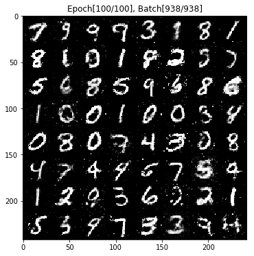
In the above code, we used
torchvision.utils.make_grid
🔗
to draw multiple images together. The
permute
🔗
method of PyTorch Tensor can be used to transform
dimensions. The running time of the entire code is
relatively long. The generator and the discriminator are
constantly in a game, and the generated images are becoming
more and more realistic. The following are the test results
generated after training for 100 epochs, and it can be seen
that they already look quite good.
64.5. Generative Adversarial Network Improvement#
The above code might make you feel extremely excited. It seems that we can build GANs through deep learning to imitate a lot of things. However, compared to convolutional neural networks being good at computer vision and recurrent neural networks being good at natural language processing, GANs don’t yet have a particularly suitable application scenario. The main reason is that there are still many problems with GANs currently. For example:
-
Non - convergence problem: GAN is a game between two neural networks. Imagine that if the discriminator learns very strongly in advance, it is very easy for the generator to experience vanishing gradients and be unable to continue learning. The convergence of all GANs has always been a problem, which also makes GANs very sensitive to various hyperparameters during actual construction and requires careful design to complete a training task.
-
Collapse problem: The GAN model is defined as a minimax problem. It can be said that GAN does not have a clear objective function. This can very easily lead to the degradation of the generator during learning, always generating the same sample points, which further causes the discriminator to always be fed the same sample points and be unable to continue learning, resulting in the collapse of the entire model.
-
The model is too free: In theory, we hope that GAN can simulate any real data distribution. However, in fact, since we do not pre - model the model, and it is a very high - probability event that “the sample spaces of the real distribution and the generated distribution do not completely overlap”. Then, for large images, if the number of pixels is too large, GAN will become increasingly uncontrollable and the training difficulty will be very high.
However, perhaps because GANs are really fascinating, in the field of deep learning in recent years, research on GANs has been surging one wave after another. New variants of GANs are constantly being proposed. For example, the Wasserstein distance is used to describe the distance between two distributions, and corresponding algorithms are designed based on the Wasserstein distance, namely WGAN.
Compared with the original GAN, the new algorithm is less sensitive to parameters and the training process is smoother. There is also CGAN, which proposes a conditional - constrained GAN. By adding restrictive conditions to the model through additional information, it guides the GAN to generate data and avoid the collapse problem. Interested students are welcome to read the [related papers](nightrome/really - awesome - gan) of GAN.

The figure above shows the change in the number of papers submitted on GANs in recent years on the well - known preprint paper website arXiv (pronounced like the English word “archive”), indicating that its popularity has been continuously rising.
64.6. The Future of Generative Adversarial Networks#
Deep learning is changing our world. Convolutional neural networks dominate the field of computer vision, enabling machines to “see” more clearly and understand better. Recurrent neural networks lead the field of natural language processing, making our machines increasingly intelligent. However, as the hottest and most trendy topic in deep learning and even the entire machine learning in the past two years, people are not particularly clear about where GAN can actually be applied. Possible applications include:
-
Augment data. That is, when the training data is not abundant enough, use GAN to generate some data to assist in the training of the model.
-
Image generation, image style transfer, image noise reduction and restoration, image super - resolution. Some good findings have been made in this regard with GAN.
-
Combine with reinforcement learning to assist intelligent machines.
We believe that GAN has provided us with a new way of thinking to solve many problems, that is, introducing game theory into the machine learning process. It can be foreseen that the algorithms of GAN itself and its perspective on problems will surely have a profound impact on future algorithm design and solving practical problems. Maybe in the future, GAN can generate our voices and generate videos with our appearances. Thinking more boldly, GAN might also be able to generate real - life scenarios as simulators to help train autonomous driving, or even generate realistic virtual visions to provide people with a brand - new gaming experience. Do these interesting ideas make you feel as if you can glimpse a bit of the future?
Maybe Inception is very close to us, or maybe the creator of Inception is you.
64.7. Summary#
This experiment introduced the currently popular GAN and attempted to use PyTorch to train a generative adversarial network for generating handwritten characters. Although GAN is interesting, it also faces many problems. This experiment is just an introduction to GAN, and in - depth research on GAN is what the academic community is currently doing. What you need to do is to understand the principle of GAN and further familiarize yourself with the use of PyTorch.
Related Links
-
[Latest Research Progress of GAN](nightrome/really - awesome - gan)
-
[Rich Application Examples of GAN](hindupuravinash/the - gan - zoo)