
59. Principles of Convolutional Neural Networks#
59.1. Introduction#
Deep learning has a wide range of applications in fields such as computer vision, and the most core models stem from the breakthrough development of convolutional neural networks. In this experiment, we will understand and learn about convolutional neural networks (CNNs) in deep learning.
59.2. Key Points#
Convolution Kernel
Convolution Stride
Padding
-
Process of High-Dimensional Convolution Kernels
-
Development History of Convolutional Neural Networks
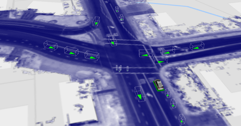
When it comes to artificial intelligence, people hope that their intelligent machines possess basic perceptual and expressive abilities like humans, such as “hearing, speaking, reading, and writing”. Computer vision is the discipline that studies how to enable machines to “see”. Nowadays, with the impetus of deep learning, computer vision has entered an era of rapid development. Face recognition, autonomous driving, medical image analysis, the maturity of computer vision has made all these possible and even far more efficient than our human work.
59.3. Overview of Convolutional Neural Networks#
In the field of computer vision, Convolutional Neural Network has played an important role. In fact, its idea source is very simple. Just as neural networks are created by simulating the working ideas of biological neurons, convolutional neural networks also simulate our vision.
In 1959, experiments by Hubel and Wiesel showed that biological visual processing starts with simple shapes such as edges, straight lines, and curves. For this discovery, Hubel and Wiesel received the Nobel Prize in Physiology or Medicine in 1981.
During the process of learning layer by layer, convolutional neural networks also simulate this process. The first layer learns relatively low-level image structures, and the second layer learns higher-level features based on the results of the first layer. In this way, the last layer can complete our learning tasks based on the high-level features learned from the previous layer.

For example, when recognizing a face, the first layer may learn simple lines, the second layer learns the contours, the second-to-last layer learns the double eyelids and earlobes, and the last layer recognizes that she is your high school head teacher. It can be said that convolutional neural networks now dominate the field of computer vision. By flexibly applying the structure of convolutional neural networks, our machines will be able to “see” more and more clearly.
Convolutional neural networks are generally feedforward neural network structures stacked by convolutional layers, pooling layers, and fully connected layers. Similar to the feedforward neural networks mentioned earlier, convolutional neural networks also use the backpropagation algorithm for training.

The figure above shows a basic convolutional neural network structure. Of course, the network structures we usually use are deeper and more complex, generally composed of many convolutional layers, pooling layers, and fully connected layers stacked crosswise, and include more additional components such as preventing overfitting.
Now let’s gradually delve deeper into convolutional neural networks. First of all, you need to understand what an image looks like in the eyes of a computer.
The following figure illustrates the concept of a pixel matrix. Specifically, what we may see is the overall visual effect of a picture, but when reading an image from a computer, the image is identified by a pixel matrix. Each pixel has a value (0 - 255), representing the magnitude of the pixel at that position in the channel of the picture.
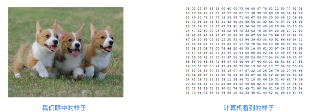
The concept of channels can be understood as colors. The commonly used RGB channels represent red, green, and blue respectively. By superimposing the pixel matrices of the three channels, the colorful pictures we see can be formed.
Therefore, in a computer, an image is a three-dimensional matrix of \(m\times n\times k\), where \(m\) is the height of the matrix, \(n\) is the width of the matrix, and \(k\) is the depth of the matrix. Based on such a data structure, convolution operations can be performed next.
59.4. Convolution Kernel (Kernel)#
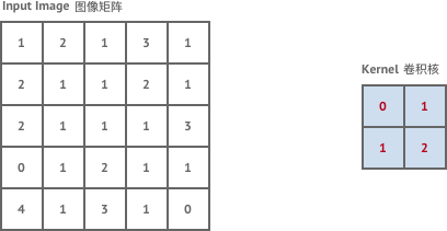
We first need to understand the concept of the convolution kernel. As shown in the following figure, on the left is the example image matrix, and on the right, a convolution kernel (weight matrix) is defined simultaneously.
Among them, the role of the convolution kernel is to extract certain features from the input matrix (image). The animation is as follows:
The above animation process is actually a convolution process. I wonder if you can understand it at a glance?
Simply put, we move the convolution kernel starting from the upper left corner of the image matrix and continuously calculate to obtain the matrix on the right. The process of convolution calculation is very simple, just multiplication and addition operations. For example, when we first place the convolution kernel at the upper left corner of the image matrix:
By continuously translating the convolution kernel and performing convolution operations with the input matrix at the same time, the convolved matrix can be obtained.
How to understand the convolution process? The simplest way is to regard the convolution kernel as a filter. After the original matrix passes through the filter, a new feature matrix is obtained.
If you want to understand vividly what the convolution kernel is actually doing, you can present the convolved image in comparison with the original image. The following figure shows the results of a picture after convolution operations with different convolution kernels. We can clearly observe that different convolution kernels can help us decompose different levels of features of the original picture.
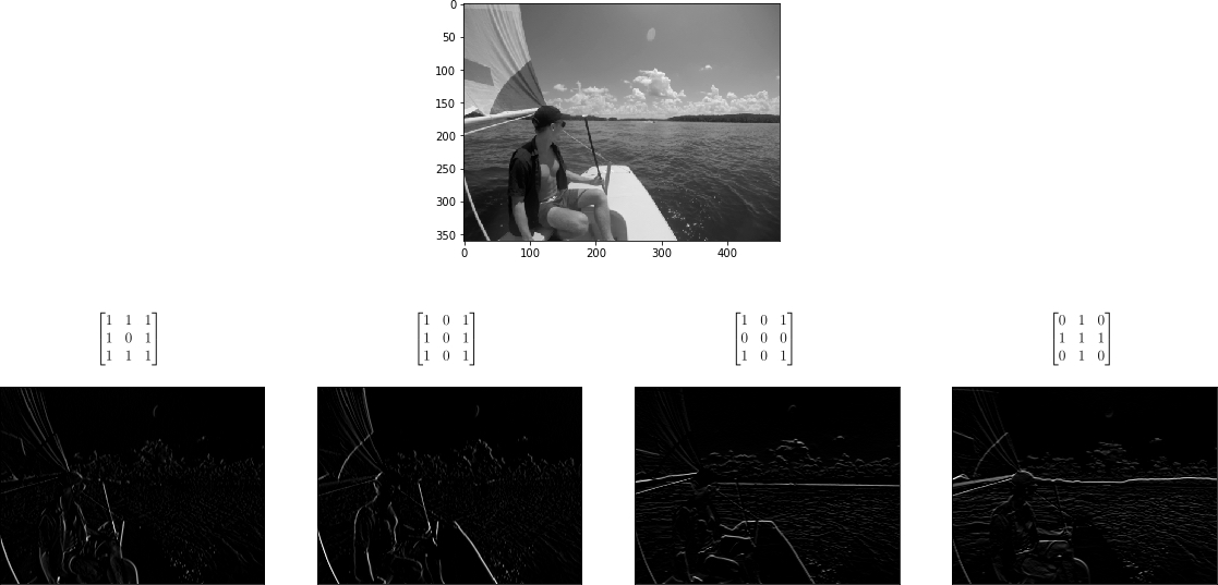
So, if the convolution kernel can help decompose image features and apply them in the process of machine learning, for example, being able to identify the details of four wheels and windows when recognizing a car, you can imagine that this will be extremely helpful in improving the accuracy.
59.5. Convolution Stride#
I believe you have understood the above convolution process. At this time, there is a question. If we move sequentially when convolving images, will the efficiency be relatively low?
Yes, for some very large images, moving only one step at a time will result in very low computational efficiency, and at the same time, the decomposed features are also prone to redundancy. Therefore, a hyperparameter can be introduced to adjust the number of steps for each movement, and we call it the convolution stride.
Similarly, we use a set of animated gifs to view the moving effects of different convolution strides:
When the convolution stride is 1, it is the same moving process as above:
At this time, the size of the output matrix is:
If we set the convolution stride to 2, the result is as follows:
It can be found that when moving horizontally and vertically with Stride = 2, one cell is skipped at each step. That is, the movement changes from one step to two steps.
At this time, the size of the output matrix (rounded down) is:
59.6. Padding#
The concept of stride has been introduced. Next, let’s introduce another important concept in the convolution operation: Padding. Padding is also known as margin. Of course, we usually directly use the English term. The stride solves the problem of low convolution efficiency, but it creates new problems. You will find that as the stride increases, the size of the convolution output matrix will continue to decrease. However, when building a network, we often hope that the size of the output matrix is a specified size and is not completely determined by the change of the convolution stride. Thus, the operation of Padding comes into being.
Once we determine the size of the original matrix and the size of the stride, the size of the resulting convolution matrix will be determined. If we want the size of the convolution matrix to be larger, without changing the size of the convolution kernel and the stride, the only way is to adjust the size of the original matrix. Thus, we achieve this goal by performing a Padding operation (expanding the margin) on the original matrix.
A common Padding operation is to add a circle of 0s around the outermost periphery of the input matrix and then participate in the convolution operation. In this way, we can control the size of the output matrix by ourselves. The following lists several common Padding methods:
Arbitrary Padding fills 0s around the input image, making the size of the output matrix larger than that of the input. For example, in the following figure, after adding two circles of 0s (dashed squares) around the periphery of the \(5\times5\) input matrix and performing a convolution operation with a \(4\times4\) convolution kernel, the process of finally obtaining a \(6\times6\) output matrix.
At this time, the size of the output matrix is:
Half Padding, also known as Same Padding, aims to obtain an output matrix with the same size as the input. The following figure shows the process of adding a circle of 0s around the periphery of a \(5\times5\) input matrix and performing a convolution operation with a \(3\times3\) convolution kernel, ultimately still obtaining a \(5\times5\) output matrix.
Another type is Full Padding. The convolution kernel starts from the first square in the upper left corner of the input matrix and moves sequentially to the last square in the lower right corner.
Actually, Padding doesn’t only have these several types. There are also some other forms, including some convolution forms that combine Padding and Stride. Even you can customize the rules of Padding and Stride, and there is no need to introduce them one by one here.
59.7. High-Dimensional Multi-Convolution Kernel Process#
Previously, we have introduced the process of a matrix passing through a single convolution kernel. I believe you are already very familiar with concepts such as convolution kernels, strides, and Padding.
A black-and-white image forms a single-pixel matrix. However, if it is a color image with RGB channels, it will form a three-dimensional pixel matrix. What should we do about this?
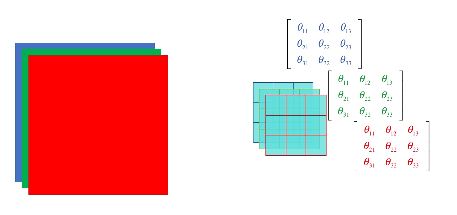
For a three-dimensional matrix of size \(m\times n\times k\), how does it operate under this two-dimensional structure convolution? In fact, there is an important principle in the design of convolutional neural networks, that is: the convolution kernel is also a three-dimensional matrix of size \(a\times b \times k\) (usually \(a = b\), and numbers like 1, 3, 5, 7 are often taken). More importantly, it must be ensured that the values of the input matrix size and the convolution kernel size are equal in the third dimension.
In this way, when we perform the above convolution operation on the input matrix and the convolution kernel with the same depth in the third dimension, we finally stack all the depth values to obtain a two-dimensional output matrix. That is to say, for an input matrix of size \(m\times n\times k\) and a convolution kernel of size \(a\times a \times k\), if we perform a convolution operation with \(\text{stride}=s\) and \(\text{padding}=p\), then we will obtain a two-dimensional matrix of size \([(m + 2p - a)/s + 1]\times [(n + 2p - a)/s + 1]\).
So how can we ensure that the output matrix is still a three-dimensional matrix? In fact, we just need to use multiple convolution kernels to perform operations in each layer. Finally, stack all the obtained two-dimensional matrices, and we will get an output matrix of size \([(m + 2p - a)/s + 1]\times [(n + 2p - a)/s + 1]\times c\), where \(c\) is the number of convolution kernels.
The whole process can be more intuitively represented by the following figure. After a \(5\times5\times3\) input matrix is convolved with two \(3\times3\times3\) convolution kernels with \(\text{stride} = 2\) and \(\text{padding} = 1\), an output matrix of size \(3\times3\times2\) is obtained:
The above is the execution process of a high-dimensional matrix through multiple convolution kernels.
The convolutional layer was introduced above. Next, another very important layer in the convolutional neural network will be introduced, namely the pooling layer. The pooling operation is actually a downsampling operation process. As we all know, images are a very large amount of training data. Therefore, only having the convolutional layer is not enough to achieve good training performance. The pooling layer compresses the images through downsampling to reduce the training parameters without affecting the image quality.
It should be noted that the pooling layer is often introduced after several convolutional layers. The pooling layer has no parameters to learn, and the pooling layer is completed independently at each depth, which means that the depth of the image remains unchanged after pooling. The following introduces two commonly used pooling methods.
59.8. Max Pooling#
For the pooling operation, we need to define a filter and a stride. In max pooling, the maximum value of the input matrix within the filter size matrix block is taken as the output at the corresponding position of the output matrix. As shown in the following figure:

59.9. Average Pooling#
In addition to max pooling, another commonly used pooling method is average pooling. As the name implies, this is to take the average value of the input matrix within the filter size matrix block as the output at the corresponding position of the output matrix. As shown in the following figure:

Compared with convolution, the process of pooling is much simpler. I believe you can clearly see the processes of max pooling and average pooling from the above schematic diagrams.
There are many techniques in the field of deep learning that require a great deal of exploration and practice. For example, for a face recognition task, the networks we build have a high degree of diversity. Under a large number of datasets and multiple experimental results, some classic neural networks have emerged. These networks have had unique superior performance and revolutionary innovative ideas since their inception. Therefore, it is recommended that everyone familiarize themselves with the architectures of these classic neural networks in the study of deep learning, which will further deepen our understanding of deep neural networks.
In fact, in the theoretical exploration of neural networks, there is not yet a very sufficient theoretical proof for why some classic networks have such powerful performance. Of course, there are still many unexplained aspects in deep learning, including what exactly each step of the neural network is learning and how each parameter affects the learning performance or the iterative convergence process. These issues all await further exploration. Therefore, the process of tuning the parameters of deep neural networks feels full of “mysticism”, which requires a large amount of practical accumulation.
59.10. LeNet Neural Network#
LeNet-5 is a very early classic convolutional neural network. Yann LeCun (known as the father of convolutional neural networks) built LeNet in 1998 and it was widely used in the handwritten recognition network (MNIST). The architecture of the LeNet neural network is as follows:
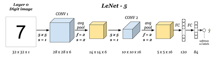
Among them, average pooling is used for downsampling in the network. The previous layers are all activated by tanh, and the last layer is activated by RBF. After testing, LeNet can reduce the error rate to 0.95% in a dataset of 60,000 original images.
Once LeNet was released, it brought a wave of convolutional neural network trends. Unfortunately, due to the limited computing power in that era, the diversity of convolutional neural networks was severely restricted. Researchers were reluctant to deepen the networks, and after a wave of enthusiasm, convolutional neural networks were almost ignored.
59.11. AlexNet Neural Network#
In the 2012 ImageNet competition, the performance of a convolutional neural network shone brightly, and this is AlexNet. After more than a decade of hardware development, the computing power of computers has increased significantly, and the data we can use has also increased significantly. Thus, AlexNet came into being.
The structure of AlexNet is very similar to LeNet-5, but the network has become larger and deeper. At the same time, AlexNet is the first network to stack convolutional layers and then pooling layers. Moreover, AlexNet uses two methods, Dropout (during training, neurons are temporarily discarded from the network with a certain probability) and data augmentation, to reduce overfitting, and LRN (local responce normalization) as a normalization layer to encourage neurons to learn more extensive features. It can be said that the excellent performance of AlexNet has gradually made the field of computer vision dominated by convolutional neural networks.
The following is the network structure diagram of AlexNet:
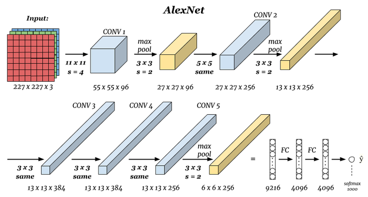
When the original author trained AlexNet, one GPU was responsible for the top part in the figure, and one GPU ran the bottom part in the figure. The GPUs only communicated with each other at certain layers. Five convolutional layers, five pooling layers, and three fully connected layers, along with approximately 50 million tunable parameters, constituted this classic convolutional neural network. The final fully connected layer output to a 1000-dimensional softmax layer, generating a distribution covering 1000 class labels. Finally, the classification task of ImageNet was completed.
59.12. VGG Neural Network#
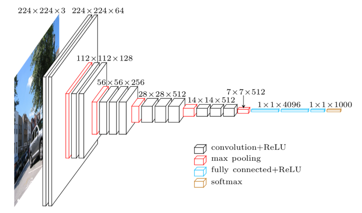
VGG Net can be regarded as a deeper version of Alex Net, and it also applies the ideas brought by Alex Net. VGG Net has 5 convolutional groups, 2 fully image-connected features, and 1 fully connected classification feature. Additionally, Alex Net has only 8 layers, while VGG Net usually has 16 to 19 layers.
The revolutionary aspect of VGG Net is that it presented different convolutional layer configuration methods in the paper. Moreover, from the experimental results in the paper, it can be seen that as the convolutional layers are gradually deepened from 8 to 16, the accuracy has reached a bottleneck value with the increase in the number of convolutional layers. This research indicates that simply adding convolutional layers often does not achieve better results, which will prompt the future development of convolutional neural networks towards the idea of enhancing the functions of convolutional layers.
The following figure depicts the VGG network structure of one configuration:
59.13. Google Net Neural Network#
After VGG Net, convolutional neural networks have evolved in another direction, which is to enhance the functions of convolutional modules.
Google Net proposed by Google can be said to have brought revolutionary results. Although at first glance it seems that the network has been made deeper, in fact, the design technique of a small module among them has enhanced the learning performance of all convolutional layers. Google calls it Inception, inspired by the contemporary movie Inception at that time. The Inception module is shown in the following figure:
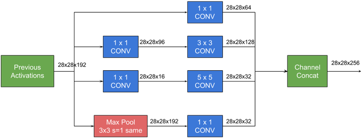
The introduction of this multi-layer perceptron convolutional layer comes from a very intuitive idea, that is, the locally sparse optimal structure in a convolutional network can often be approximated or replaced by a simple and reusable dense combination. Just like the combination of the \(1\times1\), \(3\times3\), \(5\times5\) convolutional layers and the \(3\times3\) pooling layer in the above figure forms an Inception. This is done for the following considerations:
-
Convolution kernels of different sizes can extract information at different scales.
-
Using \(1\times1\), \(3\times3\), \(5\times5\) makes alignment convenient. Padding can be 0, 1, 2 respectively for alignment.
-
Due to the successful application of the pooling layer in the CNN network, the pooling layer is also regarded as part of the combination, and its effectiveness is also demonstrated in the GoogleNet paper.
Since Google Net is a stack of several Inception modules, and generally the later Inception modules can extract more advanced and abstract features.
After the previous layer is dimension-reduced by the \(1\times1\) or pooling layer, in the fully connected layer, the filters connect the convolution results of \(1\times1\), \(3\times3\), and \(5\times5\), which can expand both the depth and width of the network. The paper shows that the Inception module accelerates the training process of the entire network by 2 to 3 times and makes it easier to capture key features for learning. At the same time, due to the very deep network, to avoid the problem of gradient vanishing, Google Net also cleverly adds two loss functions at different depths for training.
The entire Google Net structure is as follows:
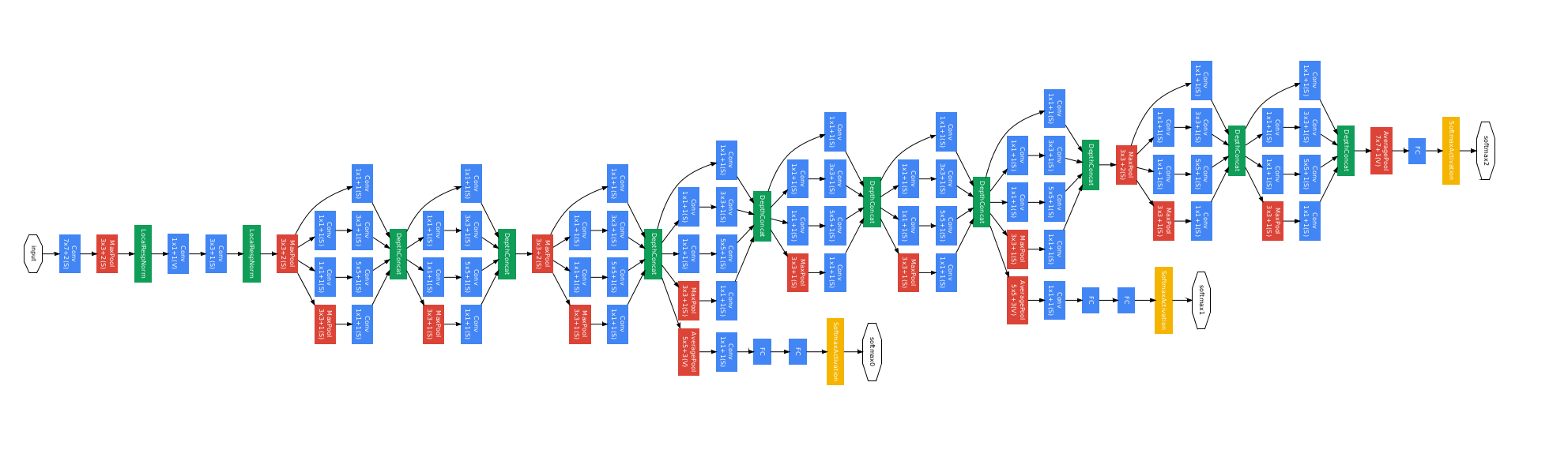
It can be seen that Google Net is already a very deep network. You can open the picture in a new tab to view the details. Both the training time and computational cost that Google Net depends on have reached a new level. This creative design of Inception has greatly optimized the learning process of convolutional neural networks.
59.14. ResNet Neural Network#
If we combine the two evolutionary directions of deepening the network and enhancing the functions of convolutional modules, ResNet is formed. ResNet, released by the team of Kaiming He in 2015, can be said to have influenced the entire deep learning community. First, let’s see how amazing this network is:
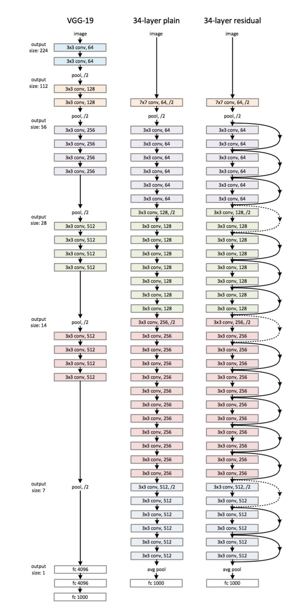
The training depth of ResNet reaches 152 layers. The figure on the right above is just a mini 34-layer ResNet structure. The figure on the left is VGG-19, and the one in the middle is a deep neural network without a Residual structure.
It can be clearly seen that ResNet performs an operation of skip-layer transmission on some parts of the network. During the process of network deepening, there may be a problem called network degradation. By introducing this skip-layer transmission, ResNet adds the result of a certain previous layer to the convolutional result of this layer to optimize a residual to avoid these problems.
ResNet multiplies the depth of our network, increasing it from a maximum of 20 layers to over 100 layers at once. Moreover, the network is no longer a normal stack of layers. Ultimately, the prediction accuracy of the model has achieved a huge quantitative improvement.
These classic neural networks are all pioneering and typical. Just like implementing AlexNet above, we can use TensorFlow to implement other networks. However, the subsequent network structures are too complex, so we will not build them by hand in the experiment. If you are interested, you can carefully study the papers of these networks according to the network structures arXiv:1512.03385 and try to build these networks by hand.
59.15. The Development History of Convolutional Neural Networks#
Finally, we use a diagram to summarize the development history of convolutional neural networks:

You may have had such a question before, that is: Why use convolutional neural networks?
Previously, neural networks such as fully connected networks, where each neuron is connected to each other and then activated, could already achieve good learning effects and could also fit to learn various complex processes. So, after the above in-depth understanding of convolutional neural networks, can you briefly answer this question?
Visually speaking, convolutional neural networks retain the spatial information of images.
In the 1960s, scientists discovered through research on the visual cortex cells of cats that each visual neuron only processes a small area of the visual image, that is, the receptive field. We also see that in a convolutional neural network, a convolutional layer can have multiple different convolutional kernels (weights), and each convolutional kernel slides on the input image and only processes a small piece of the image each time.
In this way, the convolutional layer at the input end can extract the most basic features in the image, such as straight lines or corners in different directions; then combine them into higher-order features, such as triangles, squares, etc.; continue to abstract and combine them to obtain facial features such as eyes, noses, and mouths; finally, combine the facial features into a face to complete the matching and recognition. During the process, the features extracted by each convolutional layer will be abstractly combined into higher-order features in the subsequent layers, and finally learn enough key features to complete the learning task.
In terms of computation, the convolutional layer has two key advantages, namely local connection and weight sharing.
Each neuron is only connected to a local area of the previous layer, and the spatial size of this connection can be regarded as the receptive field of the neural network neuron. The significance of weight sharing is that each layer of neurons in the current layer in the depth direction uses the same weights and biases.
A reasonable assumption is made here: If a feature is useful when calculating at a certain spatial position \((x, y)\), then it is also useful when calculating at another different position \((x_2, y_2)\). By combining local connection and weight sharing, we reduce the number of parameters and greatly decrease the training complexity. Such an operation can also mitigate overfitting, and weight sharing also endows the convolutional network with tolerance to translation.
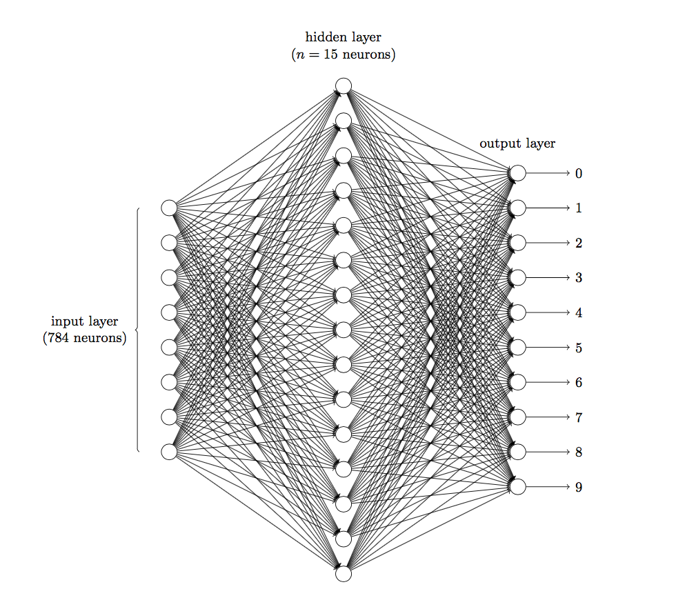
Imagine that if we use a fully connected neural network to perform an image recognition task. The picture is composed of pixel points and represented by a matrix, a \(28\times28\) matrix. We have to “flatten” it and turn it into a column vector of 784. If this column vector is connected to 15 neurons in the hidden layer, there will be \(784\times15 = 11760\) weights \(w\). If the hidden layer is connected to 10 neurons in the final output layer, there will be \(150\times10 = 1500\) weights \(w\). Finally, adding 15 bias terms in the hidden layer and 10 bias terms in the output layer, we get \(11760 + 150 + 15 + 10 = 11935\) parameters. This is really terrifying.
The following figure shows the structure of a three-layer fully connected network, with an input of an image, i.e., 784 neurons, a hidden layer of 15 neurons, and an output layer of 10 neurons:
So, imagine if we use a convolutional neural network to solve it. In the convolutional layer, we only need to learn the convolutional kernels (weights). In the pooling layer, we don’t need to learn any parameters. The number of parameters to be learned is significantly reduced compared to the above three-layer fully connected layer. This is the advantage of the convolutional neural network.
59.16. Summary#
In this experiment, we learned about the structure of convolutional neural networks, especially the principles and working methods of convolutional layers and pooling layers. Compared with fully connected neural networks, convolutional neural networks introduce the receptive field in bionics and achieve multi-layer feature extraction of images through convolutional operations. In addition, weight sharing reduces the training parameters required by neural networks and greatly improves the computational efficiency of deep neural networks.
Related Links