
57. Building Neural Networks with PyTorch#
57.1. Introduction#
Nowadays, we have learned about tensors and their operations in PyTorch, but that’s far from enough. In this experiment, we will learn how to conveniently build neural network models using PyTorch, as well as the steps and methods for training neural networks in PyTorch.
57.2. Key Points#
Building Neural Networks with PyTorch
Sequential Container Structure
Accelerating Training with GPU
Model Saving and Inference
The convenient definition of different types of Tensors and the Autograd mechanism that facilitates backpropagation are important features of deep learning frameworks. However, what truly brings great convenience is the already encapsulated different neural network structure components, including different types of layers, as well as various loss functions, activation functions, optimizers, etc.
The components for building neural network structures in
PyTorch are in
torch.nn
🔗.
Most of these neural network layers appear as classes. For
example, the fully connected layer:
torch.nn.Linear()
🔗, the MSE loss function class:
torch.nn.MSELoss()
🔗, etc.
In addition, there are also neural network layers,
activation functions, loss functions, etc. under
torch.nn.functional
🔗, but they all appear as functions. For example, the fully
connected layer function:
torch.nn.functional.linear()
🔗, the MSE loss function:
torch.nn.functionalmse_loss()
🔗, etc.
In short,
torch.nn
contains neural network component classes (capital letters),
while
torch.nn.functional
contains neural network component functions (lowercase
letters).
57.3. Building Neural Networks with PyTorch#
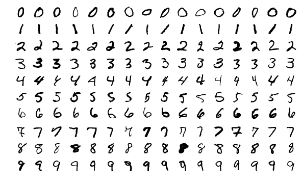
The dataset used in this experiment is MNIST. You can consider it as an enhanced version of the DIGITS dataset, both for the handwritten character task. We have used the Fashion MNIST dataset before. The MNIST dataset has the same sample features as it, only the sample categories are different. Each sample in MNIST is a \(28 \times 28\) matrix, and the target is the characters 0 - 9.
We can directly use the computer vision enhancement module
torchvision
provided by PyTorch to load the MNIST dataset.
import torchvision
import warnings

warnings.filterwarnings("ignore")

# 加载训练数据,参数 train=True,供 60000 条
train = torchvision.datasets.MNIST(
    root=".", train=True, transform=torchvision.transforms.ToTensor(), download=True
)
# 加载测试数据,参数 train=False,供 10000 条
test = torchvision.datasets.MNIST(
    root=".", train=False, transform=torchvision.transforms.ToTensor(), download=True
)
Downloading http://yann.lecun.com/exdb/mnist/train-images-idx3-ubyte.gz
Downloading http://yann.lecun.com/exdb/mnist/train-images-idx3-ubyte.gz to ./MNIST/raw/train-images-idx3-ubyte.gz
Extracting ./MNIST/raw/train-images-idx3-ubyte.gz to ./MNIST/raw

Downloading http://yann.lecun.com/exdb/mnist/train-labels-idx1-ubyte.gz
Downloading http://yann.lecun.com/exdb/mnist/train-labels-idx1-ubyte.gz to ./MNIST/raw/train-labels-idx1-ubyte.gz
Extracting ./MNIST/raw/train-labels-idx1-ubyte.gz to ./MNIST/raw

Downloading http://yann.lecun.com/exdb/mnist/t10k-images-idx3-ubyte.gz
Downloading http://yann.lecun.com/exdb/mnist/t10k-images-idx3-ubyte.gz to ./MNIST/raw/t10k-images-idx3-ubyte.gz
Extracting ./MNIST/raw/t10k-images-idx3-ubyte.gz to ./MNIST/raw

Downloading http://yann.lecun.com/exdb/mnist/t10k-labels-idx1-ubyte.gz
Downloading http://yann.lecun.com/exdb/mnist/t10k-labels-idx1-ubyte.gz to ./MNIST/raw/t10k-labels-idx1-ubyte.gz
Extracting ./MNIST/raw/t10k-labels-idx1-ubyte.gz to ./MNIST/raw
In the above code,
transform=torchvision.transforms.ToTensor()
🔗
uses the
transforms
provided by torchvision to directly convert the original
NumPy array into a PyTorch tensor. Now, you can try to
output the features and targets of the training and test
data for viewing.
train.data.shape, train.targets.shape, test.data.shape, test.targets.shape
(torch.Size([60000, 28, 28]),
 torch.Size([60000]),
 torch.Size([10000, 28, 28]),
 torch.Size([10000]))
Next, we also need to use a component provided by PyTorch to
encapsulate the data.
torch.utils.data.DataLoader
🔗
is a very commonly used data loader provided by PyTorch. It
can encapsulate the dataset into an iterator to facilitate
subsequent operations such as mini-batch loading and data
shuffling. After the data loader is prepared, we only need
to use it through a
for
loop later.
import torch

# 训练数据打乱,使用 64 小批量
train_loader = torch.utils.data.DataLoader(dataset=train, batch_size=64, shuffle=True)
# 测试数据无需打乱,使用 64 小批量
test_loader = torch.utils.data.DataLoader(dataset=test, batch_size=64, shuffle=False)
train_loader, test_loader
(<torch.utils.data.dataloader.DataLoader at 0x121141720>,
 <torch.utils.data.dataloader.DataLoader at 0x1211412a0>)
Next, we will learn the classic method of building neural networks in PyTorch, which is also a method recommended by the official.
First, a basic class
torch.nn.Module
in
torch.nn
🔗. This class is the base class for all neural networks in
PyTorch. It can represent either a single layer in a neural
network or a neural network consisting of several layers.
The various classes in
torch.nn
are actually extended by inheriting from
torch.nn.Modules. Therefore, in actual use, we can inherit from
nn.Module
to write custom network layers.
Therefore, when we build a neural network, we also need to
inherit from
torch.nn.Module. We are going to build a fully connected network with two
hidden layers.
Input (784) → Fully Connected Layer 1 (784, 512) → Fully Connected Layer 2 (512, 128) → Output (10)
import torch.nn as nn
import torch.nn.functional as F


class Net(nn.Module):
    def __init__(self):
        super(Net, self).__init__()
        self.fc1 = nn.Linear(784, 512)  # 784 是因为训练是我们会把 28*28 展平
        self.fc2 = nn.Linear(512, 128)  # 使用 nn 类初始化线性层(全连接层)
        self.fc3 = nn.Linear(128, 10)

    def forward(self, x):
        x = F.relu(self.fc1(x))  # 直接使用 relu 函数,也可以自己初始化一个 nn 下面的 Relu 类使用
        x = F.relu(self.fc2(x))
        x = self.fc3(x)  # 输出层一般不激活
        return x
We define a new neural network structure class
Net(), and combine three linear layers (fully connected layers)
using
nn.Linear. During the forward propagation, the code uses the RELU
activation function provided by the commonly used function
module
torch.nn.functional
in PyTorch. In fact, you can also achieve the same effect by
instantiating
nn.Relu.
Next, we instantiate the custom neural network class:
model = Net()
model
Net(
  (fc1): Linear(in_features=784, out_features=512, bias=True)
  (fc2): Linear(in_features=512, out_features=128, bias=True)
  (fc3): Linear(in_features=128, out_features=10, bias=True)
)
The advantage of PyTorch is that there is no need to create a session like in TensorFlow. So you can initialize a sample of random values with a length of 784 and input it into the network to test the output:
model(torch.randn(1, 784))
tensor([[-0.0389,  0.1782, -0.1142,  0.2357, -0.0486, -0.0084,  0.1878,  0.0997,
         -0.0697, -0.0907]], grad_fn=<AddmmBackward0>)
Currently, we have built the forward propagation network. The following steps are very similar to those in TensorFlow: define the loss function, optimizer, and start training.
loss_fn = nn.CrossEntropyLoss()  # 交叉熵损失函数
opt = torch.optim.Adam(model.parameters(), lr=0.002)  # Adam 优化器
Here, we choose the very commonly used cross-entropy loss
function
nn.CrossEntropyLoss
🔗, and the Adam optimizer
torch.optim.Adam
🔗. It is worth noting that in PyTorch, the optimizer needs
to be passed the parameters of the model
model.parameters(), which is a usage feature of PyTorch.
Next, we can start training, and this part of the code is very important.
def fit(epochs, model, opt):
    print("Start training, please be patient.")
    # 全数据集迭代 epochs 次
    for epoch in range(epochs):
        # 从数据加载器中读取 Batch 数据开始训练
        for i, (images, labels) in enumerate(train_loader):
            images = images.reshape(-1, 28 * 28)  # 对特征数据展平,变成 784
            labels = labels  # 真实标签
            outputs = model(images)  # 前向传播
            loss = loss_fn(outputs, labels)  # 传入模型输出和真实标签
            opt.zero_grad()  # 优化器梯度清零,否则会累计
            loss.backward()  # 从最后 loss 开始反向传播
            opt.step()  # 优化器迭代
            # 自定义训练输出样式
            if (i + 1) % 100 == 0:
                print(
                    "Epoch [{}/{}], Batch [{}/{}], Train loss: {:.3f}".format(
                        epoch + 1, epochs, i + 1, len(train_loader), loss.item()
                    )
                )
        # 每个 Epoch 执行一次测试
        correct = 0
        total = 0
        for images, labels in test_loader:
            images = images.reshape(-1, 28 * 28)
            labels = labels
            outputs = model(images)
            # 得到输出最大值 _ 及其索引 predicted
            _, predicted = torch.max(outputs.data, 1)
            correct += (predicted == labels).sum().item()  # 如果预测结果和真实值相等则计数 +1
            total += labels.size(0)  # 总测试样本数据计数
        print(
            "============ Test accuracy: {:.3f} =============".format(correct / total)
        )
fit(epochs=1, model=model, opt=opt) # 训练 1 个 Epoch,预计持续 10 分钟
Start training, please be patient.
Epoch [1/1], Batch [100/938], Train loss: 0.360
Epoch [1/1], Batch [200/938], Train loss: 0.329
Epoch [1/1], Batch [300/938], Train loss: 0.223
Epoch [1/1], Batch [400/938], Train loss: 0.120
Epoch [1/1], Batch [500/938], Train loss: 0.186
Epoch [1/1], Batch [600/938], Train loss: 0.098
Epoch [1/1], Batch [700/938], Train loss: 0.149
Epoch [1/1], Batch [800/938], Train loss: 0.073
Epoch [1/1], Batch [900/938], Train loss: 0.214
============ Test accuracy: 0.965 =============
There are detailed comments in the code above, but there are still a few points worth noting.
First, since PyTorch does not provide a flattening class
like Flatten, we use the
reshape
operation to flatten the input of
\(28 \times 28\)
into 784 to match the network structure parameters. You can
also use
view, but the official recommends using
reshape
more
🔗.
Secondly, the step
opt.zero_grad()
is very crucial. Since gradients accumulate by design in
PyTorch, we need to manually zero them out to achieve
passing in a Batch, calculating gradients, and then updating
the parameters, so that the parameter updates later won’t be
affected by the accumulated gradients from the previous
steps. However, there is a reason for PyTorch to be designed
this way. For example, when we want to increase the size of
the Batch but the hardware can’t handle a large amount of
data, we can use the gradient accumulation mechanism to wait
until multiple Batches are passed in, then update the
parameters and perform zeroing out. This gives more
flexibility to developers. Also, this feature may be
utilized in subsequent recurrent neural networks.
57.4. Sequential Container Structure#
Above, we learned the classic method steps for building a
neural network model using PyTorch. You will find that
PyTorch is a bit easier to use than TensorFlow, mainly
reflected in the convenience of the
DataLoader
data loader and debugging the forward propagation process,
as well as not having to manage sessions, etc. However,
PyTorch seems to be a bit more complex than Keras,
especially when it comes to manually constructing the
training process and paying attention to additional steps
such as executing
opt.zero_grad().
Actually, since PyTorch does not provide a higher-level API
like
tf.keras, it cannot achieve the same level of convenience as Keras.
However, we can use the Sequential network structure
provided by PyTorch to optimize the above classical process,
making the part of the neural network structure definition
more concise.
Above, we defined the network structure
Net()
class by inheriting from
nn.Module. In fact, using
nn.Sequential
🔗
can make this process more intuitive and convenient. You can
directly add the component classes required by the network
to the
Sequential
container structure in sequence.
model_s = nn.Sequential(
    nn.Linear(784, 512),  # 线性类
    nn.ReLU(),  # 激活函数类
    nn.Linear(512, 128),
    nn.ReLU(),
    nn.Linear(128, 10),
)
model_s # 查看网络结构
Sequential(
  (0): Linear(in_features=784, out_features=512, bias=True)
  (1): ReLU()
  (2): Linear(in_features=512, out_features=128, bias=True)
  (3): ReLU()
  (4): Linear(in_features=128, out_features=10, bias=True)
)
Next, we directly use the loss function and training function defined above to complete the model optimization and iteration process. Since the optimizer needs to pass in the parameters of the model, it needs to be modified to the Sequential model defined later here.
opt_s = torch.optim.Adam(model_s.parameters(), lr=0.002)  # Adam 优化器
fit(epochs=1, model=model_s, opt=opt_s)  # 训练 1 个 Epoch
Start training, please be patient.
Epoch [1/1], Batch [100/938], Train loss: 0.384
Epoch [1/1], Batch [200/938], Train loss: 0.476
Epoch [1/1], Batch [300/938], Train loss: 0.208
Epoch [1/1], Batch [400/938], Train loss: 0.160
Epoch [1/1], Batch [500/938], Train loss: 0.193
Epoch [1/1], Batch [600/938], Train loss: 0.064
Epoch [1/1], Batch [700/938], Train loss: 0.113
Epoch [1/1], Batch [800/938], Train loss: 0.065
Epoch [1/1], Batch [900/938], Train loss: 0.193
============ Test accuracy: 0.966 =============
57.5. Accelerating Training with GPU#
The Graphics Processing Unit (GPU) is an important hardware for accelerating the training of deep learning. When we build a neural network using TensorFlow, the GPU is generally automatically called without modifying the code 🔗. However, using the GPU for acceleration in PyTorch is a bit more troublesome. We need to convert both the data tensors and the model to the CUDA type 🔗. To facilitate everyone in using the GPU when using PyTorch, the general process is given below for reference.
First, we need to verify whether PyTorch can use the
available GPU for accelerated computing.
torch.cuda.is_available()
🔗
returns
True
if the GPU is available, and
False
means that only the CPU can be used.
torch.cuda.is_available()
False
Since the current environment only has a CPU,
False
is returned above, but it does not affect the learning of
the content in this section.
Generally, we will write a conditional statement in advance to ensure that the code can execute properly in both CPU and GPU environments.
# 如果 GPU 可用则使用 CUDA 加速,否则使用 CPU 设备计算
dev = torch.device("cuda") if torch.cuda.is_available() else torch.device("cpu")
dev
device(type='cpu')
Then modify the code by adding
.to(dev)
after the data and the model. In this way, PyTorch can
automatically determine whether to use GPU acceleration.
First, add
.to(dev)
after each batch of data loaded from the
DataLoader. We follow the code in
fit(epochs,
                      model,
                      opt)
.
def fit(epochs, model, opt):
    print("Start training, please be patient.")
    for epoch in range(epochs):
        for i, (images, labels) in enumerate(train_loader):
            images = images.reshape(-1, 28 * 28).to(dev)  # 添加 .to(dev)
            labels = labels.to(dev)  # 添加 .to(dev)
            outputs = model(images)
            loss = loss_fn(outputs, labels)
            opt.zero_grad()
            loss.backward()
            opt.step()
            if (i + 1) % 100 == 0:
                print(
                    "Epoch [{}/{}], Batch [{}/{}], Train loss: {:.3f}".format(
                        epoch + 1, epochs, i + 1, len(train_loader), loss.item()
                    )
                )
        correct = 0
        total = 0
        for images, labels in test_loader:
            images = images.reshape(-1, 28 * 28).to(dev)  # 添加 .to(dev)
            labels = labels.to(dev)  # 添加 .to(dev)
            outputs = model(images)
            _, predicted = torch.max(outputs.data, 1)
            correct += (predicted == labels).sum().item()
            total += labels.size(0)
        print(
            "============ Test accuracy: {:.3f} =============".format(correct / total)
        )
Next, add
.to(dev)
to the model so that the model can automatically determine
whether to use CUDA acceleration. Note that since the
optimizer is passed the model’s parameters, and these
parameters may change to the CUDA type due to the GPU, we
need to re-execute the optimizer code to prevent errors due
to inconsistent data types.
model_s.to(dev)
opt_s = torch.optim.Adam(model_s.parameters(), lr=0.002)
Finally, complete the training. If there is a GPU, the speed will be significantly better than that of the CPU.
fit(epochs=1, model=model_s, opt=opt_s) # 训练 1 个 Epoch
Start training, please be patient.
Epoch [1/1], Batch [100/938], Train loss: 0.010
Epoch [1/1], Batch [200/938], Train loss: 0.050
Epoch [1/1], Batch [300/938], Train loss: 0.036
Epoch [1/1], Batch [400/938], Train loss: 0.088
Epoch [1/1], Batch [500/938], Train loss: 0.177
Epoch [1/1], Batch [600/938], Train loss: 0.124
Epoch [1/1], Batch [700/938], Train loss: 0.150
Epoch [1/1], Batch [800/938], Train loss: 0.129
Epoch [1/1], Batch [900/938], Train loss: 0.130
============ Test accuracy: 0.976 =============
57.6. Model Saving and Inference#
We can also save a PyTorch model for inference. Simply use
torch.save
🔗
to save the model to a
.pt
file.
torch.save(model_s, "./model_s.pt")
Next, use
torch.load
🔗
to load the model and then you can use the model for
inference.
model_s = torch.load("./model_s.pt")
model_s
Sequential(
  (0): Linear(in_features=784, out_features=512, bias=True)
  (1): ReLU()
  (2): Linear(in_features=512, out_features=128, bias=True)
  (3): ReLU()
  (4): Linear(in_features=128, out_features=10, bias=True)
)
We use the first sample in the test data as an example for inference.
# 对测试数据第一个样本进行推理,注意将张量类型转换为 FloatTensor
result = model_s(test.data[0].reshape(-1, 28 * 28).type(torch.FloatTensor).to(dev))
torch.argmax(result)  # 找到输出最大值索引即为预测标签
tensor(7)
Print the true label of the first test sample.
test.targets[0] # 第一个测试数据真实标签
tensor(7)
Actually, there are other methods and applicable scenarios for saving PyTorch models, such as using a model trained on CPU in a GPU environment for inference, etc. For more details, I hope you can take some time to study the corresponding chapter in the official documentation 🔗 later.
57.7. Summary#
In this experiment, we learned how to build a network
structure by inheriting from the neural network base class
torch.nn.Module
in PyTorch, and demonstrated the complete process of using
PyTorch for model training through MNIST. This is the most
common method for building artificial neural networks using
PyTorch, and you must master it firmly. Of course, at the
end of the experiment, we also learned how to use
nn.Sequential
to build a model container, as well as PyTorch model saving
and GPU accelerated computing, etc. Subsequently, it is
recommended that you combine the examples in the PyTorch
official documentation to deeply understand and master the
application of this framework.
Related Links