Pro Membership

Pro Membership is a membership plan created by the author to maintain and update this tutorial. You can get more benefits and services, click to view details.

56. Basic Concepts and Syntax of PyTorch

56.1. Introduction

PyTorch is a deep learning framework developed mainly by Facebook. It is favored by many large companies and researchers due to its efficient computing process and good usability. In May 2018, PyTorch officially announced the integration of the functions of Caffe2 and ONNX, which is an update that the industry has been looking forward to. In this experiment, we will get familiar with PyTorch as a whole and deeply learn the use of common components.

56.2. Key Points

• Tensor Types and Definitions

• Indexing, Slicing, and Transformation

• Internal Structure of Tensors

• Automatic Differentiation (Autograd)

• Comparison of Deep Learning Frameworks

56.3. Overview of PyTorch

In addition to Google’s TensorFlow, the PyTorch framework developed mainly by Facebook is also becoming increasingly popular. Deep learning frameworks are generally similar, and concepts such as tensors, computational graphs, automatic differentiation, and neural network components are basically available. Ultimately, the purpose of neural learning frameworks is to facilitate developers to quickly build networks and complete model training.

Therefore, as a deep learning framework, PyTorch actually provides two core functions:

• Highly efficient tensor computations, while also supporting powerful GPU-accelerated computing capabilities.

• Building deep neural networks, a network structure built on top of an automatic differentiation system.

Actually, it is similar to the core functions of TensorFlow. Next, let’s learn about the main modules of PyTorch. Compared with TensorFlow, the PyTorch modules are much more concise and clear.

Package	Description
torch	Tensor computation component, compatible with NumPy arrays and with strong GPU acceleration support
torch.autograd	Automatic differentiation component, which is the core feature of PyTorch and supports all differentiable tensor operations in torch
torch.nn	Deep neural network component for flexibly building deep neural networks with different architectures
torch.optim	Optimization computation component, including common parameter optimization methods such as SGD, RMSProp, LBFGS, Adam, etc.
torch.multiprocessing	Multiprocess management component, facilitating the sharing of views of the same data in different processes
torch.utils	Utility function component, containing common functions such as data loading and training
torch.legacy(.nn/.optim)	Backward compatibility component, containing transplanted legacy code

56.4. Tensor Types and Definitions

As we all know, tensors play the role of air in deep learning. Every input and output in the neural network structure is actually a computational process for tensors. Therefore, the most core component of PyTorch is the tensor computation component. One of the greatest features of PyTorch tensors is their compatibility with NumPy arrays and strong GPU acceleration support. So, if you are familiar with NumPy, it will be much easier to get started.

Next, let’s learn how to define tensors in PyTorch and perform operations on them. First, introduce the Tensor types supported in PyTorch. Currently, PyTorch provides 7 Tensor types supported by CPU and 8 Tensor types supported by GPU, which are respectively: 🔗

Data type dtype	CPU Tensor	GPU Tensor
32-bit floating point	torch.FloatTensor	torch.cuda.FloatTensor
64-bit floating point	torch.DoubleTensor	torch.cuda.DoubleTensor
16-bit half-precision floating point	N/A	torch.cuda.HalfTensor
8-bit unsigned integer (0~255)	torch.ByteTensor	torch.cuda.ByteTensor
8-bit signed integer (-128~127)	torch.CharTensor	torch.cuda.CharTensor
16-bit signed integer	torch.ShortTensor	torch.cuda.ShortTensor
32-bit signed integer	torch.IntTensor	torch.cuda.IntTensor
64-bit signed integer	torch.LongTensor	torch.cuda.LongTensor

Among them, the default torch.Tensor type is 32-bit floating point, that is, torch.FloatTensor.

import torch as t
import warnings

warnings.filterwarnings("ignore")

t.Tensor().dtype

torch.float32

If you want to specify the global Tensor type to make the code writing more convenient, you can complete it through configuration. For example:

t.set_default_tensor_type("torch.DoubleTensor")
t.Tensor().dtype

torch.float64

At this time, the torch.Tensor type is changed to 64-bit floating point.

Of course, the most commonly used is the default torch.Tensor(), that is, torch.FloatTensor(). Let’s restore the configuration:

t.set_default_tensor_type("torch.FloatTensor")
t.Tensor().dtype

torch.float32

After talking about the types of Tensors supported in PyTorch, let’s take a look at how to create Tensors. Of course, the most basic way is to pass in a list to create:

t.Tensor([1, 2, 3])

tensor([1., 2., 3.])

Remember that PyTorch tensors are compatible with NumPy arrays as mentioned above? We can also directly create tensors from NumPy arrays.

import numpy as np

t.Tensor(np.random.randn(3))

tensor([ 1.2694, -0.9152, -0.1893])

Consistent with Numpy, you can view the shape of a Tensor through shape:

t.Tensor([[1, 2], [3, 4], [5, 6]]).shape

torch.Size([3, 2])

Similar to NumPy, PyTorch also has many other methods to quickly create specific types of Tensors:

Method	Description
ones(*sizes)	Create a Tensor filled with 1s
zeros(*sizes)	Create a Tensor filled with 0s
eye(*sizes)	Create a Tensor with 1s on the diagonal and 0s elsewhere
arange(s, e, step)	Create a Tensor from s to e with a step size of step
linspace(s, e, steps)	Create a Tensor from s to e, evenly divided into steps parts
rand/randn(*sizes)	Create a Tensor with a uniform/standard distribution
normal(mean, std)	Create a Tensor with a normal distribution
randperm(m)	Create a Tensor with a random permutation

Remember how to view the values of tensors and perform operations in TensorFlow? If we don’t enable Eager Execution, we need to initialize variables and create a new session every time to execute. PyTorch is much more convenient. It can be as intuitive as using NumPy. If you have a basic knowledge of using NumPy, you can quickly transition and learn to use PyTorch to process tensors.

56.5. Mathematical Operations

After learning the fancy creation methods of Tensors, let’s take a look at the basic operations of Tensors. First of all, two Tensors can be directly added or subtracted from each other, but their shapes must be the same:

a = t.Tensor([[1, 2], [3, 4]])
b = t.Tensor([[5, 6], [7, 8]])

print(a + b)
print(a - b)

tensor([[ 6.,  8.],
        [10., 12.]])
tensor([[-4., -4.],
        [-4., -4.]])

In addition, we can perform operations such as summation, mean, and standard deviation on Tensors. Specifically, it includes:

Method	Description
mean / sum / median / mode	Mean / Sum / Median / Mode
norm / dist	Norm / Distance
std / var	Standard Deviation / Variance
cumsum / cumprod	Cumulative Sum / Cumulative Product

Method	Description
abs / sqrt / div / exp / fmod / log / pow	Absolute Value / Square Root / Division / Exponentiation / Modulo / Power…
cos / sin / asin / atan2 / cosh	Trigonometric Functions
ceil / round / floor / trunc	Ceiling / Rounding / Floor / Truncation (keep only the integer part)
clamp(input, min, max)	Truncate the parts exceeding min and max
sigmod / tanh	Commonly used activation functions

Note that most of the time, we need to use the dim= parameter to specify the dimension of the operation, just like the axis= parameter in NumPy.

# 对 a 求列平均
a.mean(dim=0)

tensor([2., 3.])

# a 中的每个元素求平方
a.pow(2)

tensor([[ 1.,  4.],
        [ 9., 16.]])

# a 中的每个元素传入 sigmoid 函数
a.sigmoid()

tensor([[0.7311, 0.8808],
        [0.9526, 0.9820]])

You can create new cells by yourself to practice the remaining methods.

56.6. Linear Algebra

Similarly, PyTorch provides common linear algebra operation methods. Specifically, they are as follows:

Method	Description
trace	Sum of diagonal elements
diag	Diagonal elements
triu / tril	Upper triangular / Lower triangular matrix
mm	Matrix multiplication
t	Transpose
inverse	Inverse matrix
svd	Singular value decomposition

Among them, mm is an abbreviation of matmul, which is the cross product of matrices.

b.mm(a), b.matmul(a)

(tensor([[23., 34.],
         [31., 46.]]),
 tensor([[23., 34.],
         [31., 46.]]))

Of course, there are still some methods not introduced here. You can refer to the official documentation when needed.

56.7. Indexing, Slicing, Transformation

Many times, we may only need to use a part of the Tensor, and then we need to use indexing and slicing operations. These two operations in PyTorch are very similar to those in NumPy, so it is very convenient for everyone to use.

c = t.rand(5, 4)
c

tensor([[0.8058, 0.2126, 0.6394, 0.2443],
        [0.6083, 0.0346, 0.5321, 0.0177],
        [0.3934, 0.8116, 0.9679, 0.3531],
        [0.8960, 0.2706, 0.8533, 0.5015],
        [0.3999, 0.1509, 0.9774, 0.6826]])

# 取第 1 行
c[0]

tensor([0.8058, 0.2126, 0.6394, 0.2443])

# 取第 1 列
c[:, 0]

tensor([0.8058, 0.6083, 0.3934, 0.8960, 0.3999])

# 取第 2, 3 行与 3, 4 列
c[1:3, 2:4]

tensor([[0.5321, 0.0177],
        [0.9679, 0.3531]])

Sometimes, we may need to change the shape of a Tensor. In NumPy, we would use Reshape or Resize, while in PyTorch, the corresponding operations are:

c.reshape(4, 5)

tensor([[0.8058, 0.2126, 0.6394, 0.2443, 0.6083],
        [0.0346, 0.5321, 0.0177, 0.3934, 0.8116],
        [0.9679, 0.3531, 0.8960, 0.2706, 0.8533],
        [0.5015, 0.3999, 0.1509, 0.9774, 0.6826]])

In addition, view() in PyTorch can also achieve a similar effect.

c.view(4, 5)

tensor([[0.8058, 0.2126, 0.6394, 0.2443, 0.6083],
        [0.0346, 0.5321, 0.0177, 0.3934, 0.8116],
        [0.9679, 0.3531, 0.8960, 0.2706, 0.8533],
        [0.5015, 0.3999, 0.1509, 0.9774, 0.6826]])

Correspondingly, the direct differences among reshape(), resize(), and view() are as follows: resize() and view() share memory with the original Tensor when performing transformations, that is, modifying one will cause the other to change accordingly. While reshape() will copy to a new memory block.

56.8. Internal Structure of Tensors

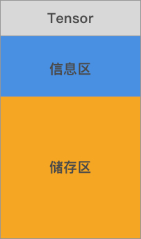
The above introduced the methods of creating, computing, and transforming Tensors. Finally, let’s take a look at the internal structure of Tensors. A PyTorch tensor is roughly composed of two parts, namely the information area (Tensor) and the storage area (Storage). Among them, the information area stores attributes such as the shape and data type of the Tensor, while the storage area holds the actual data.

Next, let’s check the data changes in the tensor storage block.

d = t.rand(3, 2)  # 生成一个随机张量
d

tensor([[0.1640, 0.8882],
        [0.2513, 0.8349],
        [0.8480, 0.8745]])

d.storage()  # 查看张量 storge 区块

 0.1639798879623413
 0.8882449865341187
 0.2513461709022522
 0.8348528146743774
 0.8480359315872192
 0.8744807839393616
[torch.storage.TypedStorage(dtype=torch.float32, device=cpu) of size 6]

d = d.reshape(2, 3)  # 改变张量的形状
d

tensor([[0.1640, 0.8882, 0.2513],
        [0.8349, 0.8480, 0.8745]])

d.storage()  # 查看改变后张量 storge 区块

 0.1639798879623413
 0.8882449865341187
 0.2513461709022522
 0.8348528146743774
 0.8480359315872192
 0.8744807839393616
[torch.storage.TypedStorage(dtype=torch.float32, device=cpu) of size 6]

As can be seen, although the size attribute of the Tensor changes, the Storage does not. Of course, what we have here is just a simple generalization and not particularly rigorous. If you want to delve deeper into the internal structure of PyTorch, you can read this article: PyTorch – Internal Architecture Tour.

That’s all for the introduction to tensors (Tensors) in PyTorch for now. In fact, you will find that the functions and methods related to Tensors in PyTorch are very similar to those of Ndarrays in NumPy. Therefore, if you master the use of Ndarrays, then there will be no problem with using Tensors.

56.9. Automatic Differentiation Autograd

Autograd automatic differentiation 🔗 is the core mechanism of PyTorch. It can automatically construct a computational graph based on the forward propagation process and automatically complete the backpropagation without having to manually implement the backpropagation process. The convenience is imaginable. Although TensorFlow also has an automatic differentiation mechanism, its design is different from that of PyTorch.

The core data structure of Autograd is torch.Tensor, which includes the following three important attributes:

• data: The data, which is the corresponding Tensor.

• grad: The gradient, which is the gradient corresponding to the Tensor. Note that grad is also a torch.Tensor object.

• grad_fn: The gradient function, which is used to construct the computational graph and automatically calculate the gradient.

Similar to the automatic differentiation process in TensorFlow, PyTorch also uses a computational graph. In particular, PyTorch is a dynamic computation graph, which allows our computational models to be more flexible and complex and enables the backpropagation algorithm to be carried out at any time.

Next, let’s calculate through an example. First, create a sample tensor.

When creating a tensor using the method provided by PyTorch, we specify requires_grad=True:

x = t.ones(3, 4, requires_grad=True)
x

tensor([[1., 1., 1., 1.],
        [1., 1., 1., 1.],
        [1., 1., 1., 1.]], requires_grad=True)

Print the data structure of torch.Tensor:

print(x.data)
print(x.grad)
print(x.grad_fn)

tensor([[1., 1., 1., 1.],
        [1., 1., 1., 1.],
        [1., 1., 1., 1.]])
None
None

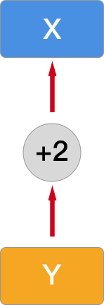
Since there is no computational process here, both grad and grad_fn are None. We can perform an operation on x:

y = x + 2
print(y)
y.grad_fn

tensor([[3., 3., 3., 3.],
        [3., 3., 3., 3.],
        [3., 3., 3., 3.]], grad_fn=<AddBackward0>)

<AddBackward0 at 0x1226f6e00>

At this point, grad_fn has traced the computational process. And the computational graph at this time is like this:

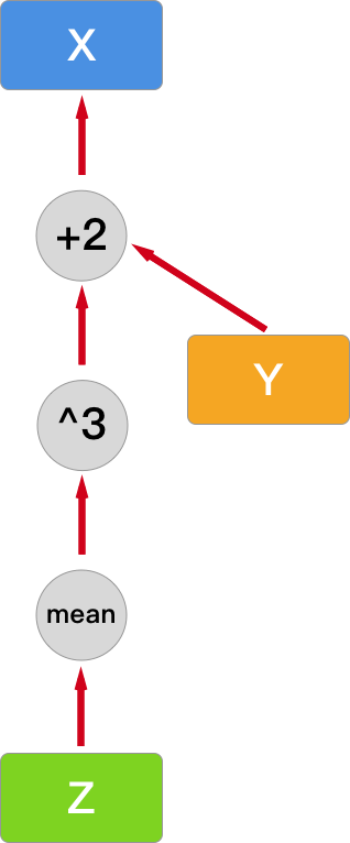
Next, we make the computational graph a bit more complex by adding a composite operation of calculating the mean here:

z = t.mean(y.pow(3))
print(z)
z.grad_fn

tensor(27., grad_fn=<MeanBackward0>)

<MeanBackward0 at 0x1226f5120>

Then, the computational graph becomes like this:

At this point, you can use backward for backpropagation and calculate the derivatives (gradients) of all leaf nodes. Note that neither Z nor Y is a leaf node, so there is no gradient information for them.

z.backward()
print(z.is_leaf, y.is_leaf, x.is_leaf)
print(z.retain_grad())
print(y.retain_grad())
print(x.retain_grad())

False False True
None
None
None

Note that since gradients are cumulative, repeatedly running the code to calculate Z is equivalent to modifying the computational graph, and the corresponding gradient values will also change. In addition, if you repeatedly run backward(), it will report an error because the required values are saved as buffers after the forward pass and are automatically cleared after the gradients are calculated. If you want to perform backpropagation multiple times, you need to use the backward(retain_graph=True) parameter to ensure the persistence of the buffers.

Next, let’s compare the process of automatic differentiation by Autograd and manual derivative calculation through another example. First, create a random Tensor and set requires_grad=True:

x = t.randn(3, 4, requires_grad=True)
x

tensor([[-0.0318, -0.9165, -0.2250, -0.6530],
        [-0.2842, -1.2158,  0.0508,  1.0140],
        [-0.0810,  0.2203,  0.2025,  0.9538]], requires_grad=True)

You may still remember the Sigmoid function and its corresponding derivative formula:

\[ g(z)=\frac{1}{1+e^{-z}} \]

\[ g(z)'=g(z)(1 - g(z)) \]

Next, manually implement the Sigmoid function and the corresponding derivative calculation function:

def sigmoid(x):
    """sigmoid 函数"""
    return 1.0 / (1.0 + t.exp(-x))


def sigmoid_derivative(x):
    """sigmoid 函数求导"""
    return sigmoid(x) * (1.0 - sigmoid(x))

y = sigmoid(x)  # 张量通过 sigmoid 计算
y

tensor([[0.4920, 0.2857, 0.4440, 0.3423],
        [0.4294, 0.2287, 0.5127, 0.7338],
        [0.4798, 0.5549, 0.5504, 0.7219]], grad_fn=<MulBackward0>)

Then, we can obtain the derivative calculation result through the Autograd mechanism. Here, we need to use backward and pass in a gradient with the same shape as y:

y.backward(gradient=t.ones(y.size()))
x.grad

tensor([[0.2499, 0.2041, 0.2469, 0.2251],
        [0.2450, 0.1764, 0.2498, 0.1953],
        [0.2496, 0.2470, 0.2475, 0.2008]])

Of course, we can manually calculate the derivative through the sigmoid_derivative() function to check the calculation result:

sigmoid_derivative(x)

tensor([[0.2499, 0.2041, 0.2469, 0.2251],
        [0.2450, 0.1764, 0.2498, 0.1953],
        [0.2496, 0.2470, 0.2475, 0.2008]], grad_fn=<MulBackward0>)

You will see that the calculation results obtained using the Autograd mechanism are the same as the manually calculated results.

In particular, PyTorch provides a special context manager torch.no_grad() for temporarily disabling the tracking of history. This context manager is usually used when evaluating a model because when evaluating a model, we don’t need to calculate gradients or update model parameters.

Here is a simple example:

z1 = x * 2
with t.no_grad():
    z2 = x * 2
    
print(z1.requires_grad, z2.requires_grad)

True False

56.10. Comparison of Deep Learning Frameworks

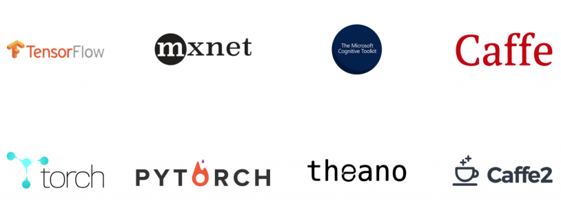
Machine之心 has an article that introduces each framework in great detail. There is no need to describe the features of each framework in too much detail here. There are many machine learning frameworks, and it is impossible to learn each one. This is unrealistic. One can only choose a framework that is more suitable for one’s own situation and of interest for in-depth learning.

MXNet and CNTK are developed by two top companies, Amazon and Microsoft respectively. Both frameworks are very excellent and easy to use, but they are not very popular. There are two questions on Zhihu specifically discussing the reasons why these two frameworks have not gained popularity. If you are interested, you can learn about this history.

• Why is the popularity and penetration rate of CNTK lower than that of TensorFlow, Theano, Caffe, and Torch?

• Why has the powerful MXNet not gained popularity?

Torch and Theano are two relatively early frameworks that have had a profound impact on the development of deep learning frameworks. Torch is developed based on the relatively niche language Lua. Theano was developed by Bengio, one of the “Big Three”, but it has stopped being maintained.

Keras is an API with a higher-level encapsulation based on TensorFlow, Theano, and CNTK. It is very easy to get started compared to other frameworks. However, precisely because of this high-level encapsulation, it is very difficult to modify the training details in Keras. Now Keras has been incorporated into TensorFlow.

Caffe is an open-source framework developed by Yangqing Jia during his PhD at UC Berkeley. Its purpose is very clear, mainly for deep learning in images. Caffe is widely used because of its very fast processing speed. Caffe’s position in the field of Computer Vision is unique. Although it is now being replaced by emerging frameworks such as TensorFlow and PyTorch, due to its accumulation, the community support for Caffe is very good. Many new ideas and articles in the CV field are implemented based on Caffe. For example, well-known Object Detection algorithms such as Fast RCNN, Faster RCNN, and SSD are all like this. Therefore, if your main research direction is computer vision, then it is also necessary for you to learn this framework. Caffe2 will be incorporated into PyTorch later because the developer has joined Facebook.

Other frameworks, such as PaddlePaddle developed by Baidu and NCNN developed by Tencent, will not be introduced in detail here. These frameworks are mostly used in internal projects or cooperation projects of related enterprises.

To sum up, the current options are two mainstream deep learning frameworks: TensorFlow and PyTorch. In this article PyTorch vs TensorFlow — spotting the difference, the two frameworks are compared in detail, perhaps more detailed than the introduction in this experiment. The two frameworks are developed by two large companies respectively, and generally speaking, both are very good.

56.10.1. Advantages of PyTorch

56.10.1.1. More user-friendly

In the Q&A on Zhihu How to evaluate the PyTorch 1.0 Roadmap?, almost all the answers are complaints about TensorFlow and praises for the ease of use of PyTorch.

The ease of use of PyTorch is specifically manifested in its easy debugging. You can directly use the most basic print or the debugger in PyCharm to step by step debug and view the output. While for TensorFlow, you need to use tfdbg, and if you want to debug native Python code, you also need to use other tools. PyTorch comes with many pre-written modules, such as data loading, preprocessing, etc., and it is very convenient for users to implement custom modules. Maybe you just need to inherit a certain class and then write a few methods. However, in TensorFlow, for each defined network, you need to declare, initialize parameters such as weights and biases, so a large amount of repetitive code needs to be written. And PyTorch provides many deep learning structures such as convolutional layers and pooling layers in the nn.Module module, with a relatively higher level of abstraction compared to TensorFlow, so it is very convenient.

56.10.1.2. Very strong code readability

The reason PyTorch is called PyTorch is that it is implemented in Python. Unless it is very low-level operations such as matrix calculations which are implemented in C/C++ and then encapsulated with Python. As we all know, the readability of Python code is not in the same league as that of C++.

For example, the torchvision module implemented in PyTorch contains a lot of image preprocessing, loading, pre-trained models, etc., all implemented in Python. You can go and read the code implementation inside. For example, image flipping, how AlexNet is implemented in PyTorch. While TensorFlow is much more troublesome.

56.10.1.3. More user-friendly documentation

PyTorch has very good API documentation and getting-started tutorials. For each implemented Loss Function, it will introduce its implementation principle, paper address, mathematical formula, etc., probably aiming to enable users to better understand the framework. There are many claims that TensorFlow has more documentation and the official getting-started tutorials are available in Chinese. But actually, for something translated by a foreign company, there will always be some problems in understanding. These documents read very strangely and are not as good as reading the original text directly.

Another drawback of TensorFlow is that its documentation is very messy. For example, in the TensorFlow Tutorial, there are several tutorials just about MNIST, which is really dazzling. While PyTorch Tutorials presents a lot of Notebooks for learning from practical applications.

56.10.2. Advantages of TensorFlow

56.10.2.1. Convenient visualization

TensorFlow’s Tensorboard is very useful and can visualize models, curves, etc. Tensorboard will save data locally for self-customized visualization.

Of course, PyTorch also has visualization tools. For example, Visdom provided by Facebook can conveniently manage many models, but it cannot export data. In addition, PyTorch can also use tensorboardX to call Tensorboard for visualization (although not all functions can be used). Generally speaking, TensorFlow is slightly stronger than PyTorch in this regard.

56.10.2.2. Convenient deployment

Whether it is server deployment or mobile deployment, PyTorch is almost completely defeated. After all, Google’s position in the field of AI is unique.

For server deployment, TensorFlow has TensorFlow Serving. For mobile deployment, TensorFlow Lite compresses the model to the extreme, with very fast running speed, supports Android and iOS. There is also TensorFlow.js that can directly call WebGL to predict models.

Of course, PyTorch has also been constantly making up for its deficiencies in this regard. After version 1.0, Caffe2 was merged into PyTorch, and JIT was introduced, etc., enabling PyTorch to also have deployment capabilities. You can view The road to 1.0: production ready PyTorch for further understanding. Of course, there are also other methods such as converting the PyTorch Model into the models of other frameworks for deployment, or you can also deploy it by yourself using Flask, Django, etc., but it is relatively troublesome.

56.10.2.3. Well-developed community

TensorFlow has a very high market share and is used by many people. There are a large number of resources, blogs, etc. on the Internet introducing TensorFlow. In contrast, PyTorch is relatively new, so there may be more English content. Now PyTorch is gradually catching up. In addition, many cloud service providers offer machine learning platforms that support TensorFlow to run cloud servers for model training, but they may not necessarily support PyTorch.

There is no perfect framework. Even after years of development, TensorFlow still has many problems. There are detailed discussions in What are the unacceptable aspects of TensorFlow? and What are the pitfalls/bugs in PyTorch?. One can only choose a suitable framework according to their own needs. When specifically discussing how to choose a framework, we will introduce it according to different groups of people:

56.10.2.4. If you are a student or a researcher

Students and researchers have more time and can spend a lot of time learning. The best option is to be familiar with both frameworks. While mainly using one framework, also have a certain understanding of the other, at least be able to understand the code.

In the academic field, various frameworks are used, but mainly concentrated in TensorFlow and PyTorch (Caffe is mainly concentrated in computer vision). If you are a student but will work in the future, or a researcher but inclined towards engineering or in need of engineering applications, then you may need to focus more on using TensorFlow. If you are a student but inclined towards scientific research, or a researcher who hopes to quickly implement their own algorithms and run a prototype, then the flexible PyTorch would be more suitable.

56.10.2.5. If you are already working

For those who are already working, time may not be充裕, so choose a framework according to your own ability and understand it deeply. To learn this course, it must be based on an interest in artificial intelligence and machine learning. If you hope to engage in this industry in the future and make a living from machine learning, then TensorFlow is the inevitable choice. If it is just based on interest and you hope to enter a new industry, then PyTorch is easier to get started with and is a better choice.

To sum up, you may need to choose a suitable framework according to your own preference. It’s not necessary to choose a certain one just as understood above. After all, a framework is just a framework, not basic knowledge. The ability to understand how the framework operates at the underlying level, such as how Batch Norm is implemented, is the most important. It is hoped that you can realize that a framework is just a tool. If you don’t understand the principle, you can only be an outsider, commonly known as a “package adjuster”.

56.11. Summary

In this section of the experiment, we learned about several of the most important components in PyTorch, which are: Tensor, Autograd, nn, and Optimizer. After understanding and mastering these components, we can complete the construction of a deep neural network. Of course, we will learn about different deep neural network structures in detail in subsequent courses. The experience accumulated in this section of the experiment is very important because you will keep using the knowledge points learned today in future experiments.

---

○ Sharethis article link to your social media, blog, forum, etc. More external links will increase the search engine ranking of this site.

If you find this content helpful, you can buy me a coffee

Previous

55. TensorFlow Fashion Item Classification

Next

57. Building Neural Networks with PyTorch