
49. Handwritten Character Recognition Neural Network#
49.1. Introduction#
In the previous experiment, we introduced the principle of artificial neural networks starting from perceptrons and elaborated in detail on the process of backpropagation in neural networks through theoretical derivations. In this challenge, we will combine the implementation method of artificial neural networks provided by scikit-learn to complete handwritten character recognition.
49.2. Key Points#
Artificial Neural Network
Handwritten Character Recognition
49.3. Overview of Handwritten Character Datasets#
In this challenge, we will use the handwritten character dataset DIGITS. The full name of this dataset is Pen-Based Recognition of Handwritten Digits Data Set, which is sourced from the UCI Open Datasets website.
The dataset contains digital matrices converted from 1,797
handwritten character images of the digits 0 to 9, and the
target values are 0 - 9. For convenience, here we directly
use the
load_digits
method provided by scikit-learn to load this dataset.
import numpy as np
from sklearn import datasets

digits = datasets.load_digits()
The loaded DIGITS dataset contains three attributes:
Attribute |
Description |
|---|---|
|
|
8x8 matrix recording the pixel grayscale values corresponding to each handwritten character image |
|
|
Converting the corresponding 8x8 matrix of
|
|
|
Recording the digits represented by each of the 1,797 images |
Next, we output the first handwritten character for viewing.
The digit corresponding to the first character image:
digits.target[0]
0
The grayscale value matrix corresponding to the first character image:
digits.images[0]
array([[ 0.,  0.,  5., 13.,  9.,  1.,  0.,  0.],
       [ 0.,  0., 13., 15., 10., 15.,  5.,  0.],
       [ 0.,  3., 15.,  2.,  0., 11.,  8.,  0.],
       [ 0.,  4., 12.,  0.,  0.,  8.,  8.,  0.],
       [ 0.,  5.,  8.,  0.,  0.,  9.,  8.,  0.],
       [ 0.,  4., 11.,  0.,  1., 12.,  7.,  0.],
       [ 0.,  2., 14.,  5., 10., 12.,  0.,  0.],
       [ 0.,  0.,  6., 13., 10.,  0.,  0.,  0.]])
Flatten the matrix into a row vector:
digits.data[0]
array([ 0.,  0.,  5., 13.,  9.,  1.,  0.,  0.,  0.,  0., 13., 15., 10.,
       15.,  5.,  0.,  0.,  3., 15.,  2.,  0., 11.,  8.,  0.,  0.,  4.,
       12.,  0.,  0.,  8.,  8.,  0.,  0.,  5.,  8.,  0.,  0.,  9.,  8.,
        0.,  0.,  4., 11.,  0.,  1., 12.,  7.,  0.,  0.,  2., 14.,  5.,
       10., 12.,  0.,  0.,  0.,  0.,  6., 13., 10.,  0.,  0.,  0.])
You may feel that numbers are always not very intuitive. Then, based on the grayscale value matrix, we can use Matplotlib to draw the grayscale image corresponding to the character.
from matplotlib import pyplot as plt

%matplotlib inline

image1 = digits.images[0]
plt.imshow(image1, cmap=plt.cm.gray_r)
<matplotlib.image.AxesImage at 0x146b52380>

It can be clearly seen from the above image that it is the handwritten character 0.
{exercise-start}
:label: chapter06_03_1
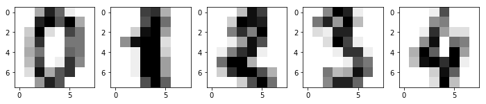
Challenge: Use the \(1 \times 5\) subplot style to draw the images of the first 5 handwritten characters in the Digits dataset.
{exercise-end}
## 代码开始 ### (3~5 行代码)


## 代码结束 ###
{solution-start} chapter06_03_1
:class: dropdown
### Code start ### (3 - 5 lines of code)
fig, axes = plt.subplots(1, 5, figsize=(12,4))
for i, image in enumerate(digits.images[:5]):
    axes[i].imshow(image, cmap=plt.cm.gray_r)
### Code end ###
{solution-end}
Expected output
Next, we need to randomly split the dataset into a training set and a test set for future use.
{exercise-start}
:label: chapter06_03_2
Challenge: Use
train_test_split()
to split the dataset into 80% (training set) and 20% (test
set).
Requirement: Define the training set features, training set
targets, test set features, and test set targets as
X_train,
                      y_train,
                      X_test,
                      y_test
respectively, and set the random seed to 30.
{exercise-end}
## 代码开始 ### (≈ 2 行代码)


## 代码结束 ###
{solution-start} chapter06_03_2
:class: dropdown
### Start of code ### (≈ 2 lines of code)
from sklearn.model_selection import train_test_split

X_train, X_test, y_train, y_test = train_test_split(digits.data, digits.target, test_size=0.2, random_state=30)
### End of code ###
{solution-end}
Run the tests
len(X_train), len(y_train), len(X_test), len(y_test), np.mean(y_test[5:13])
Expected output
(1437, 1437, 360, 360, 3.75)
49.4. Building an Artificial Neural Network with scikit-learn#
The
MLPClassifier()
class in scikit-learn implements a multi-layer neural
network structure with the backpropagation algorithm.
sklearn.neural_network.MLPClassifier(hidden_layer_sizes=(100, ), activation='relu', solver='adam', alpha=0.0001, batch_size='auto', learning_rate='constant', learning_rate_init=0.001, power_t=0.5, max_iter=200, shuffle=True, random_state=None, tol=0.0001, verbose=False, warm_start=False, momentum=0.9, nesterovs_momentum=True, early_stopping=False, validation_fraction=0.1, beta_1=0.9, beta_2=0.999, epsilon=1e-08)
This class has many parameters. We introduce the main parameters as follows:
- hidden_layer_sizes: Defines the number of hidden layers and the number of neurons they contain. (20, 20) represents 2 hidden layers with 20 neurons each.
- activation: The activation function, with options including identity (linear), logistic, tanh, relu.
- solver: The solution method, with options including lbfgs (quasi - Newton method), sgd (stochastic gradient descent), adam (improved sgd). Adam works well on relatively large datasets (thousands of samples). For small datasets, lbfgs converges faster and has good results.
- alpha: The regularization term parameter.
- learning_rate: The learning rate adjustment strategy, with options including constant (unchanged), invscaling (gradually decreasing), adaptive (adaptive).
- learning_rate_init: The initial learning rate, used to update the weights during stochastic gradient descent.
- max_iter: The maximum number of iterations.
- shuffle: Determines whether to reshuffle the samples at each iteration.
- random_state: The random number seed.
- tol: The tolerance for optimization solution. When the difference in loss between two iterations is less than this tolerance, the model considers it to have converged and training stops.
Next, we are going to build a neural network prediction
model using
MLPClassifier().
Exercise 49.1
Challenge: Use
MLPClassifier()
to build a neural network structure, train a handwritten
character recognition model, and finally obtain the
prediction accuracy on the test set.
Requirements:
-
The neural network structure contains
2hidden layers, with100and50neurons respectively. -
Use
reluas the activation function. -
Use the stochastic gradient descent
SGDmethod for solution. -
The learning rate is
0.02and remains unchanged during the learning process. -
The maximum number of iterations is
100times. -
Set the random number seed to
1. -
Use default values for the remaining parameters.
from sklearn.neural_network import MLPClassifier
from sklearn.metrics import accuracy_score


def mpl():
    """
    参数:无

    返回:
    model -- 人工神经网络模型
    score -- 测试集上的预测准确率
    """
    ### 代码开始 ### (≈ 2 行代码)
    model = None

    score = None
    ### 代码结束 ###
    return model, score
Solution to Exercise 49.1
from sklearn.neural_network import MLPClassifier
from sklearn.metrics import accuracy_score

def mpl():
    """
    Parameters: None

    Returns:
    model -- The artificial neural network model
    score -- The prediction accuracy on the test set
    """
    ### Code starts ### (≈ 2 lines of code)
    model = MLPClassifier(
        hidden_layer_sizes=(100, 50),
        activation='relu',
        solver='sgd',
        learning_rate_init=0.02,
        learning_rate='constant',
        max_iter=100,
        random_state=1
    )

    model.fit(X_train, y_train)
    score = accuracy_score(y_test, model.predict(X_test))
    ### Code ends ###
    return model, score
Run the test
mpl()[1]
Expected output
> 0.95
The general accuracy of the neural network trained with the
above parameters can reach about 98%. We can output some
attributes of the
model, such as the number of iterations and plot the curve of
the change of the loss during iteration.
# 绘制损失变化曲线
model = mpl()[0]
plt.plot(model.loss_curve_)
# 输出模型达到收敛的迭代次数
model.n_iter_