Pro Membership

Pro Membership is a membership plan created by the author to maintain and update this tutorial. You can get more benefits and services, click to view details.

36. Time Series Data Analysis and Processing

36.1. Introduction

Time series is a data type often encountered in data analysis. Understanding and mastering relevant features and processing methods can help us handle time series analysis tasks. In this experiment, we focus on learning a series of preprocessing techniques for time series using Pandas.

36.2. Key Points

• Time generation

• Time conversion

• Time calculation

• Time zone

• Timestamp

• Timestamp index

• Time series retrieval

• Time series offset

• Resampling

Time series analysis is often encountered in the process of data analysis, especially in financial data analysis. A time series is a set of random variables sorted by time. For example, the GDP or CPI index regularly released by the National Bureau of Statistics every year or month; the numerical changes of stocks, funds, and indexes over a period of time are all time series.

The following figure shows the stock price change curve of Google for only 5 years. In fact, this curve is drawn from the daily closing prices, which is a typical time series dataset.

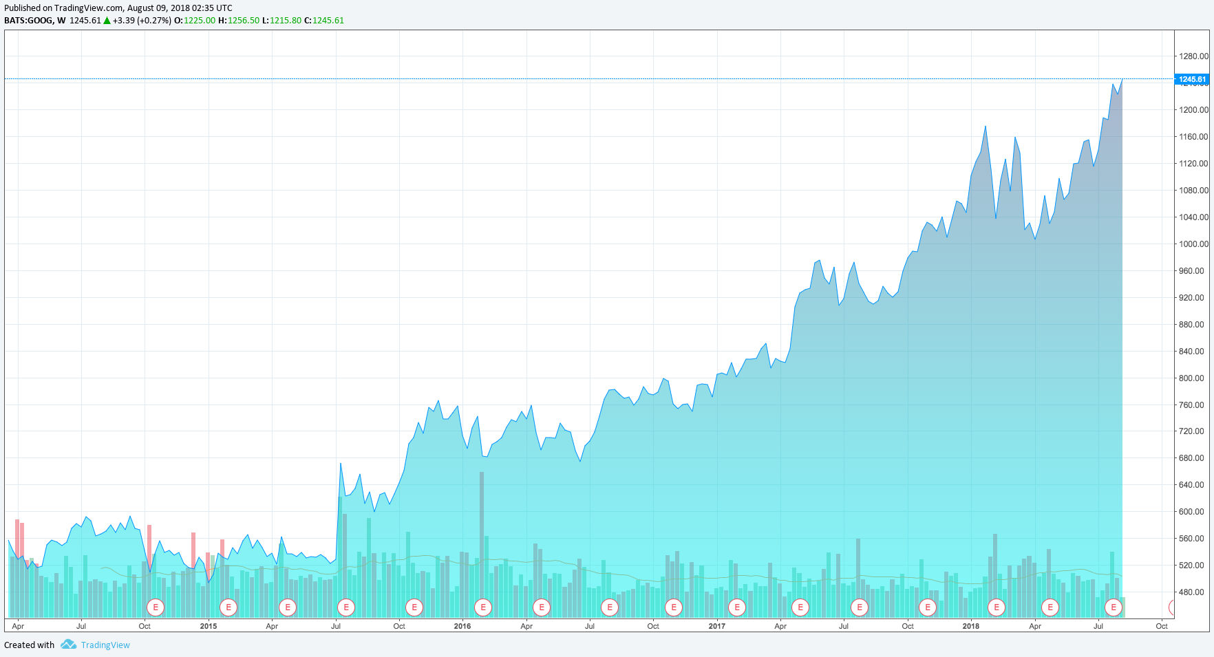
In addition to the financial field, time series are widely present in other aspects such as the environment and physics. For example, the air quality index changes over time, and server log data is generated over time.

Similarly, Pandas provides a series of standard time series processing tools and algorithms, which are essential for processing and analyzing time series using Python. Next, we will learn about time generation, time series generation, indexing, slicing, sampling, etc.

36.3. Time Generation

Before learning about time series, it is necessary to understand time first. In Python, we usually use the datetime and time modules to perform time operations. For example, datetime.datetime.now can print the current time.

import datetime

datetime.datetime.now()  # 获取当前时间

datetime.datetime(2023, 11, 11, 13, 36, 28, 1146)

As can be seen, datetime.datetime.now() returns a time object, which are in sequence: year, month, day, hour, minute, second, and microsecond. Among them, the value range of microsecond is 0 <= microsecond < 1000000. There is an equivalent method for datetime.datetime.now(), which is datetime.datetime.today().

datetime.datetime.today()  # 获取当前时间

datetime.datetime(2023, 11, 11, 13, 36, 28, 15287)

You can choose to return only a part of the time.

datetime.datetime.now().year  # 返回当前年份

2023

In addition to getting the current time, you can manually specify a time object.

datetime.datetime(2017, 10, 1, 10, 59, 30)  # 指定任意时间

datetime.datetime(2017, 10, 1, 10, 59, 30)

36.4. Time Calculation

datetime time objects can be involved in calculations. For example, adding a certain amount of time and years, calculating year intervals, etc.

datetime.datetime(2018, 10, 1) - datetime.datetime(2017, 10, 1)  # 计算时间间隔

datetime.timedelta(days=365)

As can be seen, the above returns a datetime.timedelta object. timedelta can be used to represent differences in time, but only up to three units are retained, namely: days, seconds, and milliseconds. For example:

datetime.datetime.now() - datetime.datetime(2017, 10, 1)  # timedelta 表示间隔时间

datetime.timedelta(days=2232, seconds=48988, microseconds=37705)

Therefore, if you want to add one year to the current time, you need to convert the number of years into days for calculation.

datetime.datetime.now() + datetime.timedelta(365)  # 需将年份转换为天

datetime.datetime(2024, 11, 10, 13, 36, 28, 41982)

36.5. Time Format Conversion

Although datetime objects are precise, there are many times when we want to convert them into custom time representation styles, such as: October 1, 2018, or 2018/10/1, etc. At this time, it is necessary to convert the datetime object into a string object.

We can use datetime.date.strftime to complete the conversion between time and string.

datetime.datetime.now().strftime("%Y-%m-%d")  # 转换为自定义样式

'2023-11-11'

datetime.datetime.now().strftime("%Y 年 %m 月 %d 日")  # 转换为自定义样式

'2023 年 11 月 11 日'

You will find that we have used placeholders. Then, the placeholders supported by strftime are:

• %y Two-digit year representation (00 - 99)

• %Y Four-digit year representation (0000 - 9999)

• %m Month (01 - 12)

• %d Day of the month (0 - 31)

• %H Hour in 24-hour format (0 - 23)

• %I Hour in 12-hour format (01 - 12)

• %M Minutes (00 - 59)

• %S Seconds (00 - 59)

• %a Local abbreviated weekday name

• %A Local full weekday name

• %b Local abbreviated month name

• %B Local full month name

• %c Local corresponding date and time representation

• %j Day of the year (001 - 366)

• %p Local equivalent of A.M. or P.M.

• %U Week number of the year (00 - 53), with Sunday as the start of the week

• %w Weekday (0 - 6), with Sunday as the start of the week

• %W Week number of the year (00 - 53), with Monday as the start of the week

• %x Local corresponding date representation

• %X Local corresponding time representation

• %Z Name of the current time zone

In addition to converting datetime objects to strings, you can also convert string time to datetime objects. This operation is mainly considered for the flexibility of datetime objects, which can be used for secondary conversion. For example, you only need to use placeholders to represent the rules of the original string, and it can be automatically converted into a datetime time object, which is very convenient.

datetime.datetime.strptime("2018-10-1", "%Y-%m-%d")

datetime.datetime(2018, 10, 1, 0, 0)

36.6. Time Zone

A time zone is a definition of an area on Earth that uses the same time. If time is expressed in Coordinated Universal Time (UTC), then we can use the UTC offset to define the time in different time zones. For example, since Beijing is in the eighth time zone east of Greenwich, Beijing time is UTC +08:00, which represents a time zone that is 8 hours ahead of Coordinated Universal Time.

Source

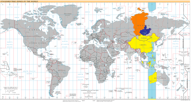
When we use datetime.now() to print the current time, it does not contain time zone information. This is also called a Naive datetime object, that is, a “naive time zone”. We can use datetime.datetime.utcnow() to get the UTC time.

datetime.datetime.utcnow()  # 获取 UTC 时间

datetime.datetime(2023, 11, 11, 5, 36, 28, 59689)

So, at this time, if you want to get Beijing time, you can add 8 hours to UTC, i.e., UTC+8:00.

utc = datetime.datetime.utcnow()  # 获取 UTC 时间
tzutc_8 = datetime.timezone(datetime.timedelta(hours=8))  # + 8 小时
utc_8 = utc.astimezone(tzutc_8)  # 添加到时区中
print(utc_8)

2023-11-11 05:36:28.063327+08:00

The time has been introduced above. If we associate the time with the collected data, a time series is formed. In a time series, there are mainly two types:

• Timestamp: A single moment.

• Time interval: Composed of a start timestamp and an end timestamp. Some time intervals can be a period, such as the year 2018, representing the time interval of the whole year.

Next, we learn the methods of using Pandas to process time series.

36.7. Timestamp

A timestamp represents a specific point in time. In Pandas, we can directly use pandas.Timestamp to create timestamps.

import pandas as pd

pd.Timestamp("2018-10-1")

Timestamp('2018-10-01 00:00:00')

Alternatively, create timestamps by combining with the datetime module.

pd.Timestamp(datetime.datetime.now())

Timestamp('2023-11-11 13:36:28.350028')

In addition, we can also use pandas.to_datetime to create timestamps. For example:

pd.to_datetime("1-10-2018")

Timestamp('2018-01-10 00:00:00')

The above code creates a timestamp for 2018-01-10 by default. What if we want it to be 2018-10-01? We can correct it by using the dayfirst=True parameter.

pd.to_datetime("1-10-2018", dayfirst=True)

Timestamp('2018-10-01 00:00:00')

36.8. DatetimeIndex for Time Index

Timestamps are not the type that is often encountered in time series. If we have a data table sorted by time, then a more important data type is the DatetimeIndex. As the name implies, a time index consists of a series of timestamps, but in Pandas, the data type is DatetimeIndex.

We can also use pd.to_datetime() to create a time index. The difference from creating timestamps above is that you only need to input a list containing multiple moments.

pd.to_datetime(["2018-10-1", "2018-10-2", "2018-10-3"])  # 生成时间索引

DatetimeIndex(['2018-10-01', '2018-10-02', '2018-10-03'], dtype='datetime64[ns]', freq=None)

Of course, the Series and DataFrame in Pandas can also be directly converted through to_datetime.

s = pd.Series(["2018-10-1", "2018-10-2", "2018-10-3"])
pd.to_datetime(s)  # 将 Seris 中字符串转换为时间

0   2018-10-01
1   2018-10-02
2   2018-10-03
dtype: datetime64[ns]

It is worth noting here that the time in the original Series is a string, and after conversion by pd.to_datetime(), it becomes a datetime64 time. However, it is not a time index in the strict sense. A time index requires placing it in the index position of the Series or DataFrame. For example:

pd.Series(index=pd.to_datetime(s)).index  # 当时间位于索引时，就是 DatetimeIndex

DatetimeIndex(['2018-10-01', '2018-10-02', '2018-10-03'], dtype='datetime64[ns]', freq=None)

Now what we see is the DatetimeIndex type.

In fact, another more commonly used method to generate a DatetimeIndex is pandas.date_range. We can specify rules to let pandas.date_range generate an ordered DatetimeIndex.

The default parameters of the date_range method are as follows:

pandas.date_range(start=None, end=None, periods=None, freq=’D’, tz=None, normalize=False, name=None, closed=None, **kwargs)

Among them:

• start=：Sets the start time

• end= ：Sets the end time

• periods=：Sets the time interval. If None, the start and end times need to be set separately.

• freq=：Sets the interval period.

• tz= ：Sets the time zone.

In particular, the freq= frequency parameter is very crucial. The available periods that can be set are:

• freq='s' : Seconds

• freq='min': Minutes

• freq='H' : Hours

• freq='D' : Days

• freq='w' : Weeks

• freq='m' : Months

• freq='BM' : Last day of each month

• freq='W' : Sundays of each week

pd.date_range("2018-10-1", "2018-10-2", freq="H")  # 按小时间隔生成时间索引

DatetimeIndex(['2018-10-01 00:00:00', '2018-10-01 01:00:00',
               '2018-10-01 02:00:00', '2018-10-01 03:00:00',
               '2018-10-01 04:00:00', '2018-10-01 05:00:00',
               '2018-10-01 06:00:00', '2018-10-01 07:00:00',
               '2018-10-01 08:00:00', '2018-10-01 09:00:00',
               '2018-10-01 10:00:00', '2018-10-01 11:00:00',
               '2018-10-01 12:00:00', '2018-10-01 13:00:00',
               '2018-10-01 14:00:00', '2018-10-01 15:00:00',
               '2018-10-01 16:00:00', '2018-10-01 17:00:00',
               '2018-10-01 18:00:00', '2018-10-01 19:00:00',
               '2018-10-01 20:00:00', '2018-10-01 21:00:00',
               '2018-10-01 22:00:00', '2018-10-01 23:00:00',
               '2018-10-02 00:00:00'],
              dtype='datetime64[ns]', freq='H')

# 从 2018-10-1 开始，以天为间隔，向后推 10 次
pd.date_range("2018-10-1", periods=10, freq="D")

DatetimeIndex(['2018-10-01', '2018-10-02', '2018-10-03', '2018-10-04',
               '2018-10-05', '2018-10-06', '2018-10-07', '2018-10-08',
               '2018-10-09', '2018-10-10'],
              dtype='datetime64[ns]', freq='D')

# 从 2018-10-1 开始，以 1H20min 为间隔，向后推 10 次
pd.date_range("2018-10-1", periods=10, freq="1H20min")

DatetimeIndex(['2018-10-01 00:00:00', '2018-10-01 01:20:00',
               '2018-10-01 02:40:00', '2018-10-01 04:00:00',
               '2018-10-01 05:20:00', '2018-10-01 06:40:00',
               '2018-10-01 08:00:00', '2018-10-01 09:20:00',
               '2018-10-01 10:40:00', '2018-10-01 12:00:00'],
              dtype='datetime64[ns]', freq='80T')

With date_range, we can generate any time index that changes according to a certain pattern.

Previously, we learned that timedelta can be used for time operations. In a DatetimeIndex, we can use offset objects to make more flexible changes to the timestamp index. For example:

1. It is possible to increase or decrease the time index by a certain time period.

2. It is possible to multiply the time index by an integer.

3. It is possible to move the time index forward or backward to the next or previous specific offset date.

time_index = pd.date_range("2018-10-1", periods=10, freq="1D1H")
time_index

DatetimeIndex(['2018-10-01 00:00:00', '2018-10-02 01:00:00',
               '2018-10-03 02:00:00', '2018-10-04 03:00:00',
               '2018-10-05 04:00:00', '2018-10-06 05:00:00',
               '2018-10-07 06:00:00', '2018-10-08 07:00:00',
               '2018-10-09 08:00:00', '2018-10-10 09:00:00'],
              dtype='datetime64[ns]', freq='25H')

Use the offset object to increase time_index by 1 month + 2 days + 3 hours in sequence.

from pandas import offsets

time_index + offsets.DateOffset(months=1, days=2, hours=3)

DatetimeIndex(['2018-11-03 03:00:00', '2018-11-04 04:00:00',
               '2018-11-05 05:00:00', '2018-11-06 06:00:00',
               '2018-11-07 07:00:00', '2018-11-08 08:00:00',
               '2018-11-09 09:00:00', '2018-11-10 10:00:00',
               '2018-11-11 11:00:00', '2018-11-12 12:00:00'],
              dtype='datetime64[ns]', freq=None)

Alternatively, use the offset object to offset time_index backward by 2 weeks.

time_index + 2 * offsets.Week()

DatetimeIndex(['2018-10-15 00:00:00', '2018-10-16 01:00:00',
               '2018-10-17 02:00:00', '2018-10-18 03:00:00',
               '2018-10-19 04:00:00', '2018-10-20 05:00:00',
               '2018-10-21 06:00:00', '2018-10-22 07:00:00',
               '2018-10-23 08:00:00', '2018-10-24 09:00:00'],
              dtype='datetime64[ns]', freq=None)

In addition to offsets.DateOffset and offsets.Week mentioned in the example, the commonly used offsets objects also include:

DateOffset Name	Description
DateOffset	Custom, default is one week
BDay	Business day
CDay	Custom business day
MonthEnd	End of month
QuarterEnd	End of quarter
YearEnd	End of year

A more detailed form of DateOffset Objects can be read in the official documentation.

You can find that the DateOffset object is very flexible. With a little combination, you can achieve any desired time offset result. In fact, the DateOffset object is not only valid for DatetimeIndex, but also can be operated on the timestamp Timestamp. This should be easy to understand, as the DatetimeIndex is equivalent to an extension of the Timestamp.

36.9. Time Intervals (Periods)

Above, we have a relatively thorough understanding of both the Timestamp and the DatetimeIndex. In addition, there are also the Period time interval and PeriodIndex time interval index objects in Pandas. What are Periods? For example: days, months, quarters, years.

# 1 年跨度
pd.Period("2018")

Period('2018', 'A-DEC')

# 1 个月跨度
pd.Period("2018-1")

Period('2018-01', 'M')

# 1 天跨度
pd.Period("2018-1-1")

Period('2018-01-01', 'D')

You will see that there is a letter after each time interval. In fact, this is the freq= frequency corresponding to the time interval. You may be thinking that Periods seems to have no difference from the above Timestamp. Then let’s regenerate a Timestamp to take a look.

pd.Timestamp("2018-1-1")

Timestamp('2018-01-01 00:00:00')

At this point, you should be able to notice the difference between Timestamp and Periods. Periods represents the entire day of 2018-01-01, while Timestamp only represents the moment of 2018-01-01 00:00:00.

36.10. PeriodsIndex (Time Interval Index)

Similar to “timestamp → time index”, time intervals also correspond to the PeriodsIndex (time interval index). And we can generate an index sequence through the pandas.period_range() method.

p = pd.period_range("2018", "2019", freq="M")  # 生成 2018-1 到 2019-1 序列，按月分布
p

PeriodIndex(['2018-01', '2018-02', '2018-03', '2018-04', '2018-05', '2018-06',
             '2018-07', '2018-08', '2018-09', '2018-10', '2018-11', '2018-12',
             '2019-01'],
            dtype='period[M]')

When generating the index sequence, it is necessary to specify the freq= frequency, which is similar to generating the DatetimeIndex above. At the same time, we can use asfreq to reset the frequency.

p.asfreq(freq="D", how="S")  # 频度从 M → D

PeriodIndex(['2018-01-01', '2018-02-01', '2018-03-01', '2018-04-01',
             '2018-05-01', '2018-06-01', '2018-07-01', '2018-08-01',
             '2018-09-01', '2018-10-01', '2018-11-01', '2018-12-01',
             '2019-01-01'],
            dtype='period[D]')

Here, how=S represents the first day of each month (Start), and it can also be set to how=E (End).

36.11. Selection, Slicing, and Shifting of Time Series Data

You may be wondering why Pandas uses timestamps, time indexes, time intervals, etc. In fact, these basic data types emerged to facilitate our operations on time series data. With Timestamp and Periods, we can complete operations such as data selection, slicing, as well as more complex combined transformations like shifting and resampling.

Next, we will try to generate an example of a Series with a time index and select data from it.

import numpy as np

timeindex = pd.date_range("2018-1-1", periods=20, freq="M")
s = pd.Series(np.random.randn(len(timeindex)), index=timeindex)
s

2018-01-31    0.330330
2018-02-28    1.087339
2018-03-31   -1.486658
2018-04-30    0.783250
2018-05-31    1.527258
2018-06-30    0.152985
2018-07-31   -0.310307
2018-08-31   -0.839569
2018-09-30   -1.905840
2018-10-31    0.542714
2018-11-30   -0.083846
2018-12-31    0.330400
2019-01-31   -0.475228
2019-02-28   -0.871950
2019-03-31   -1.174331
2019-04-30    0.095896
2019-05-31    0.353876
2019-06-30    0.159181
2019-07-31    0.759272
2019-08-31   -1.708107
Freq: M, dtype: float64

Select all the data for the year 2018.

s["2018"]

2018-01-31    0.330330
2018-02-28    1.087339
2018-03-31   -1.486658
2018-04-30    0.783250
2018-05-31    1.527258
2018-06-30    0.152985
2018-07-31   -0.310307
2018-08-31   -0.839569
2018-09-30   -1.905840
2018-10-31    0.542714
2018-11-30   -0.083846
2018-12-31    0.330400
Freq: M, dtype: float64

Select all the data between July 2018 and March 2019.

s["2018-07":"2019-03"]

2018-07-31   -0.310307
2018-08-31   -0.839569
2018-09-30   -1.905840
2018-10-31    0.542714
2018-11-30   -0.083846
2018-12-31    0.330400
2019-01-31   -0.475228
2019-02-28   -0.871950
2019-03-31   -1.174331
Freq: M, dtype: float64

In addition to querying and slicing, we can also use the Shifting method to shift the time index as a whole.

s.shift(3)  # 时间索引以默认 Freq: M 向后偏移 3 个单位

2018-01-31         NaN
2018-02-28         NaN
2018-03-31         NaN
2018-04-30    0.330330
2018-05-31    1.087339
2018-06-30   -1.486658
2018-07-31    0.783250
2018-08-31    1.527258
2018-09-30    0.152985
2018-10-31   -0.310307
2018-11-30   -0.839569
2018-12-31   -1.905840
2019-01-31    0.542714
2019-02-28   -0.083846
2019-03-31    0.330400
2019-04-30   -0.475228
2019-05-31   -0.871950
2019-06-30   -1.174331
2019-07-31    0.095896
2019-08-31    0.353876
Freq: M, dtype: float64

You can understand the above process as shifting the time index backward (into the future) by 3 units, and Pandas will automatically fill the missing data with NaN. In addition, you can also specify the freq= parameter to determine the unit size of the shift.

s.shift(-3, freq="D")  # 时间索引以 Freq: D 向前偏移 3 个单位

2018-01-28    0.330330
2018-02-25    1.087339
2018-03-28   -1.486658
2018-04-27    0.783250
2018-05-28    1.527258
2018-06-27    0.152985
2018-07-28   -0.310307
2018-08-28   -0.839569
2018-09-27   -1.905840
2018-10-28    0.542714
2018-11-27   -0.083846
2018-12-28    0.330400
2019-01-28   -0.475228
2019-02-25   -0.871950
2019-03-28   -1.174331
2019-04-27    0.095896
2019-05-28    0.353876
2019-06-27    0.159181
2019-07-28    0.759272
2019-08-28   -1.708107
dtype: float64

36.12. Resampling of Time Series Data

Resampling is an operation often used in the processing of time series data. The purpose of resampling is to increase or decrease the frequency of a time-indexed sequence. For example: when the volume of time series data is very large, we can obtain a new dataset with a smaller scale but still relatively comprehensive time coverage through the method of low-frequency sampling. In addition, resampling can be a very important means when data alignment is required for multiple datasets with different frequencies.

Similarly, initialize a sample Series.

dateindex = pd.period_range("2018-10-1", periods=20, freq="D")
s = pd.Series(np.random.randn(len(dateindex)), index=dateindex)
s

2018-10-01   -0.375011
2018-10-02    1.052191
2018-10-03   -0.232303
2018-10-04   -1.632577
2018-10-05   -0.362599
2018-10-06   -0.866722
2018-10-07   -0.244350
2018-10-08    1.501014
2018-10-09    0.558769
2018-10-10   -2.173344
2018-10-11    0.112917
2018-10-12    2.078360
2018-10-13    1.596991
2018-10-14   -0.098130
2018-10-15   -0.175248
2018-10-16    0.184979
2018-10-17   -0.223399
2018-10-18    0.427384
2018-10-19    0.170283
2018-10-20   -0.234324
Freq: D, dtype: float64

Next, we downsample the Series by 2 days and sum the data corresponding to the 2 days as the new data. Note that when performing downsampling using pandas.DataFrame.resample, a calculation method (sum, average, maximum, minimum, etc.) needs to be selected.

s.resample("2D").sum()  # 降采样，并将删去的数据依次合并到保留数据中

2018-10-01    0.677181
2018-10-03   -1.864881
2018-10-05   -1.229321
2018-10-07    1.256664
2018-10-09   -1.614575
2018-10-11    2.191277
2018-10-13    1.498861
2018-10-15    0.009731
2018-10-17    0.203986
2018-10-19   -0.064040
Freq: 2D, dtype: float64

Well, if you don’t want to operate on the data corresponding to the data index during downsampling, but only retain the data corresponding to the original timestamps, you can use the .asfreq() method.

s.resample("2D").asfreq()  # 降采样，直接舍去数据

2018-10-01   -0.375011
2018-10-03   -0.232303
2018-10-05   -0.362599
2018-10-07   -0.244350
2018-10-09    0.558769
2018-10-11    0.112917
2018-10-13    1.596991
2018-10-15   -0.175248
2018-10-17   -0.223399
2018-10-19    0.170283
Freq: 2D, dtype: float64

It can also be done like this. Downsample by 2 days and list the original values, maximum values, minimum values, etc. of the data corresponding to the 2 days. This method is mainly used in stock analysis, where open, high, low, and close correspond to the opening price, highest price, lowest price, and closing price during the stock trading process.

s.resample("2D").ohlc()

	open	high	low	close
2018-10-01	-0.375011	1.052191	-0.375011	1.052191
2018-10-03	-0.232303	-0.232303	-1.632577	-1.632577
2018-10-05	-0.362599	-0.362599	-0.866722	-0.866722
2018-10-07	-0.244350	1.501014	-0.244350	1.501014
2018-10-09	0.558769	0.558769	-2.173344	-2.173344
2018-10-11	0.112917	2.078360	0.112917	2.078360
2018-10-13	1.596991	1.596991	-0.098130	-0.098130
2018-10-15	-0.175248	0.184979	-0.175248	0.184979
2018-10-17	-0.223399	0.427384	-0.223399	0.427384
2018-10-19	0.170283	0.170283	-0.234324	-0.234324

In addition to downsampling, upsampling is also feasible. However, when considering upsampling, what should we do about the values corresponding to the timestamps newly added to the time index? Should we use the adjacent data or fill it with other methods?

For example, we can increase the time frequency from days to hours and fill the newly added rows with the same data.

s.resample("H").ffill()  # 升采样，使用相同的数据对新增加行填充

2018-10-01 00:00   -0.375011
2018-10-01 01:00   -0.375011
2018-10-01 02:00   -0.375011
2018-10-01 03:00   -0.375011
2018-10-01 04:00   -0.375011
                      ...   
2018-10-20 19:00   -0.234324
2018-10-20 20:00   -0.234324
2018-10-20 21:00   -0.234324
2018-10-20 22:00   -0.234324
2018-10-20 23:00   -0.234324
Freq: H, Length: 480, dtype: float64

Control the maximum number of fillings by setting limit=, and the values that are not filled will be automatically marked as NaN.

s.resample("H").ffill(limit=3)  # 升采样，最多填充临近 3 行

2018-10-01 00:00   -0.375011
2018-10-01 01:00   -0.375011
2018-10-01 02:00   -0.375011
2018-10-01 03:00   -0.375011
2018-10-01 04:00         NaN
                      ...   
2018-10-20 19:00         NaN
2018-10-20 20:00         NaN
2018-10-20 21:00         NaN
2018-10-20 22:00         NaN
2018-10-20 23:00         NaN
Freq: H, Length: 480, dtype: float64

36.13. Time Series Data Time Zone Processing

Above, we learned about time zone processing in datetime, and time zone processing may also occur in Pandas. Similar to datetime, the time series in Pandas is still naive in terms of time zone.

naive_time = pd.date_range("1/10/2018 9:00", periods=10, freq="D")
naive_time

DatetimeIndex(['2018-01-10 09:00:00', '2018-01-11 09:00:00',
               '2018-01-12 09:00:00', '2018-01-13 09:00:00',
               '2018-01-14 09:00:00', '2018-01-15 09:00:00',
               '2018-01-16 09:00:00', '2018-01-17 09:00:00',
               '2018-01-18 09:00:00', '2018-01-19 09:00:00'],
              dtype='datetime64[ns]', freq='D')

Therefore, when we need to convert to local time, we need to first add UTC time zone information to the time series and then convert it to local time.

utc_time = naive_time.tz_localize("UTC")
utc_time

DatetimeIndex(['2018-01-10 09:00:00+00:00', '2018-01-11 09:00:00+00:00',
               '2018-01-12 09:00:00+00:00', '2018-01-13 09:00:00+00:00',
               '2018-01-14 09:00:00+00:00', '2018-01-15 09:00:00+00:00',
               '2018-01-16 09:00:00+00:00', '2018-01-17 09:00:00+00:00',
               '2018-01-18 09:00:00+00:00', '2018-01-19 09:00:00+00:00'],
              dtype='datetime64[ns, UTC]', freq='D')

Next, we use the tz_localize method to achieve time zone conversion.

utc_time.tz_convert("Asia/Shanghai")

DatetimeIndex(['2018-01-10 17:00:00+08:00', '2018-01-11 17:00:00+08:00',
               '2018-01-12 17:00:00+08:00', '2018-01-13 17:00:00+08:00',
               '2018-01-14 17:00:00+08:00', '2018-01-15 17:00:00+08:00',
               '2018-01-16 17:00:00+08:00', '2018-01-17 17:00:00+08:00',
               '2018-01-18 17:00:00+08:00', '2018-01-19 17:00:00+08:00'],
              dtype='datetime64[ns, Asia/Shanghai]', freq='D')

Note that generally when we define UTC+8:00, we use Asia/Chongqing or Asia/Shanghai, not Asia/Beijing. This is due to historical reasons.

In fact, when generating timestamps or time indices, you can specify the tz= parameter to define the UTC time zone.

pd.date_range("1/10/2018 9:00", periods=10, freq="D", tz="Asia/Shanghai")

DatetimeIndex(['2018-01-10 09:00:00+08:00', '2018-01-11 09:00:00+08:00',
               '2018-01-12 09:00:00+08:00', '2018-01-13 09:00:00+08:00',
               '2018-01-14 09:00:00+08:00', '2018-01-15 09:00:00+08:00',
               '2018-01-16 09:00:00+08:00', '2018-01-17 09:00:00+08:00',
               '2018-01-18 09:00:00+08:00', '2018-01-19 09:00:00+08:00'],
              dtype='datetime64[ns, Asia/Shanghai]', freq='D')

However, it should be noted that due to the change in the reference of UTC time (tz= will take the specified time as UTC), the result of the previous line is different from the conversion result through tz_convert before.

36.14. Summary

A time series is nothing but a series of data sampled at time points, with a simple form. In this experiment, we learned about the basic elements of time series data in Pandas and the methods and techniques for Pandas to handle time series data. Only by mastering these methods can we better work with time series data and extract valuable information from it.

---

○ Sharethis article link to your social media, blog, forum, etc. More external links will increase the search engine ranking of this site.

If you find this content helpful, you can buy me a coffee

Previous

35. Association Rule Analysis of Shopping Data

Next

37. Stock Time Series Data Processing