
34. Apriori Association Rule Learning Method#
34.1. Introduction#
Association rule learning is a method for discovering interesting relationships between variables in large databases. Its purpose is to identify strong rules found in the database using some interesting measures. Association rules are widely used in basket analysis, web usage mining, intrusion detection, continuous production, and bioinformatics.
34.2. Key Points#
Association rules
Frequent itemsets
Support
Confidence
Example shopping data
Association rule tasks
Apriori algorithm
Association rule practice
34.3. Association Rules#
Association Rule is a means and method in data mining to discover interesting relationships between variables. Its main purpose is to find the relevance and strong rules in data. Simply put, when the frequency of a certain category of data or a certain pattern increases in a dataset, naturally everyone will think that it may be more common or important. Then, if it is found that two or more categories of data appear simultaneously, it can naturally be considered that there is a connection or rule between them.
The most typical example of association rules is used for shopping basket analysis. Some merchants find that when customers buy product A, they are very likely to buy product B at the same time. So they can adjust the placement of products or change the pricing strategy accordingly. Here is a story about beer and diapers: Generally speaking, the sales team of a large supermarket found that young American men who bought diapers on Friday afternoons also had the tendency to buy beer. So every Friday, a diaper shelf was placed next to the beer shelf, and as a result, the sales of both increased.

This example above is used in almost every article about “association analysis”. So, how did the sales team discover this purchasing pattern? It involves the use of “association analysis”.
Before formally introducing the relevant algorithms involved in association analysis, let’s first clarify several concepts commonly encountered in the process of association analysis.
34.4. Frequent Item Sets#
First, let’s understand the concept of an item set. Suppose there is a set \(I\) as follows:
Then, we call \(i_1, i_2,..., i_m\) in it the items of the set, and \(I\) is naturally called the set of items.
At this time, if the set \(S\) satisfies \(S = \{i|i ∈ I\}\), then \(S\) is called an itemset of \(I\). Among them, an itemset containing \(k\) items is called a \(k\)-itemset.
For example, when we go shopping in a supermarket, if there are many categories of goods in our shopping cart, the shopping cart can be regarded as the set \(I\). At this time, if there is beer and diapers in the shopping cart, then beer and diapers can form an itemset \(S\) of the set \(I\). If we consider all the bills of the whole supermarket in a day as the set \(I\), then the set of goods that appear in a single shopping cart can be regarded as the itemset \(S\).
A frequent itemset indicates that an itemset appears very “frequently”. From an intuitive perspective, you should think that mining frequent itemset is meaningful. For example, the above “beer and diapers”, because they appear with a high frequency, and ultimately we can benefit by adjusting the sales rules.
However, how to measure the “frequency” in a frequent itemset? To what extent can it be called “frequent”?
In association rules, we usually use expressions like \(X → Y\). Among them, \(X\) and \(Y\) are disjoint item sets, that is, \(X\cap Y = ∅\). The strength of an association rule can be measured by its support and confidence.
34.5. Support#
Support is used to measure the frequency of an event occurring. \(support(X \to Y)\) represents the frequency of the itemset \(\{X, Y\}\) in the total itemset \(I\), denoted as:
If we still take supermarket shopping as an example. In the above formula, \(support(X \to Y)\) represents the percentage of shopping carts that contain both product \(X\) and \(Y\) in the total number of shopping carts. For example, if \(X\) represents beer and \(Y\) represents diapers. Then, we count the number of shopping carts that contain both beer and diapers, divide the result by the total number of shopping carts to get the support of this itemset. If the support of an itemset exceeds a pre-set minimum support threshold, then this itemset is considered potentially useful and is called a “frequent itemset”.
34.6. Confidence#
Confidence is used to represent the likelihood of \(Y\) occurring given that \(X\) has occurred. Its formula is:
Then, \(confidence(X \to Y)\) represents the probability that \(Y\) occurs given that \(X\) has occurred. That is, the probability that diapers appear when beer appears in the shopping cart. Confidence is the percentage of shopping carts that contain both \(X\) and \(Y\) divided by the percentage of shopping carts that contain only \(X\).
In short, support represents the probability that \(X\) and \(Y\) occur simultaneously, while confidence represents the probability that \(Y\) also occurs given that \(X\) has occurred, that is, the conditional probability \(P(Y|X)\).
With support and confidence, frequent itemsets can be extended to association rules. That is to say, if we have a rule as follows:
-
\(support(Beer \to Diaper) = 10\%\)
-
\(confidence(Beer \to Diaper) = 60\%\)
That is to say, in the supermarket’s sales records, 10% of the customers’ shopping carts contain the combination of beer and diapers. At the same time, there is a 60% chance that customers who buy beer will also buy diapers. The left side of the association rule is the determined item, called the antecedent. The right side is the resulting item, called the consequent.
34.7. Example Shopping Data#
To help everyone become familiar with the relevant concepts in association rules, we will next set a group of example data and try to calculate the support and confidence of several rules.
Shopping Cart |
Item |
Item |
Item |
Item |
Item |
|---|---|---|---|---|---|
Cart A |
Milk |
Coffee |
- |
- |
- |
Cart B |
Coke |
Coffee |
Milk |
Beer |
- |
Cart C |
Beer |
Diaper |
Milk |
- |
- |
Cart D |
Coffee |
Milk |
Banana |
Sprite |
Beer |
Cart E |
Beer |
Diaper |
Coffee |
- |
- |
In the above table, there are records of 5 shopping carts. Next, we specify the rule as: \(\{Milk, Coffee\} \rightarrow \{Beer\}\)
First, the support count of the itemset \(\{Milk, Coffee, Beer\}\) is 2, and the total count is 5. So:
Since the support count of the itemset \(\{Milk, Coffee\}\) is 3, the confidence of this rule is:
That is to say, 40% of the customers bought milk, coffee, and beer at the same time. Among the customers who bought milk and coffee, the probability of buying beer is 67%.
Regarding the support and confidence of a rule. The significance of support is to help us determine whether this rule is worthy of attention. That is to say, we usually directly ignore the rules with low support. At the same time, the significance of confidence is to help us determine the reliability of the rule, whether there is enough data indicating that this rule is likely to exist.
34.8. Association Rule Task#
In the above content, we learned the representation method of association rules and three related concepts involved in a single rule. In fact, association rule mining is to discover rules whose support and confidence are greater than the thresholds we set from numerous item sets.
The above sentence may sound simple, but as you can imagine, it is not easy to implement at all. Because in real situations, the datasets we face are much more complex than the example data we presented above. Then, for the combinations of different item sets, the number of rule combinations will become extremely large. More specifically, the total number of possible rules extracted from a dataset containing \(n\) items is (a permutation and combination problem):
For example, for the dataset containing 5 different products above, 180 different rules can be combined, which is \(3^5 - 2^{5 + 1}+1\). For the item set {milk, coffee, beer}, 12 different rules can be combined, which is \(3^3 - 2^{3 + 1}+1\):
Although the itemset \(\{Milk, Coffee, Beer\}\) can generate the 12 rules above, the latter 6 rules can also be regarded as being generated by its subsets \(\{Milk, Coffee\}\), \(\{Milk, Beer\}\), and \(\{Coffee, Beer\}\). For these 12 rules, the support of the first 6 is the same, and the support between any two of the latter 6 with the same itemset is the same. Since the calculation method of support only relates to the frequency of the itemset appearing in the dataset. Then, if the itemset \(\{Milk, Coffee, Beer\}\) is a non-frequent itemset, the first 6 rules can be directly pruned without calculating their confidence, thus saving computational overhead.
That is to say, the mining of association rules is decomposed into two subtasks:
-
Discover frequent itemsets: Discover all itemsets that meet the minimum support threshold, which are the so-called “frequent itemsets”.
-
Calculate association rules: Extract all rules with high confidence from the discovered frequent itemsets as the results of association rule mining.
34.9. Apriori Algorithm#
We usually use the “lattice structure” to enumerate the possible itemsets in the dataset. As shown in the following lattice structure diagram, the possible itemsets generated by the dataset consisting of Milk, Coffee, and Beer are as follows:

As mentioned above, in the dataset consisting of Milk, Coffee, and Beer, 7 candidate itemsets (itemsets composed of single items) may be generated. Generalizing to the general case, for a dataset containing \(n\) items, \(2^n - 1\) candidate itemsets may be generated.
So, when we want to find frequent itemsets from candidate itemsets. A brute-force approach is to calculate the support count for each candidate itemset, but as \(n\) increases, the computational overhead can be imagined. Thus, there is a method of using the Apriori principle to reduce the number of candidate itemsets.
The Apriori algorithm first appeared in the paper Fast algorithms for mining association rules in large databases in 1994, and it is also the most commonly used method in association rule mining.
The Apriori principle is very simple. It mainly tells us two theorems, namely:
-
Theorem 1: If an itemset is a frequent itemset, then all of its subsets must also be frequent itemsets.
-
Theorem 2: If an itemset is an infrequent itemset, then all of its supersets must also be infrequent itemsets.
The following figure presents a lattice structure diagram of candidate itemsets that is larger than the above example.
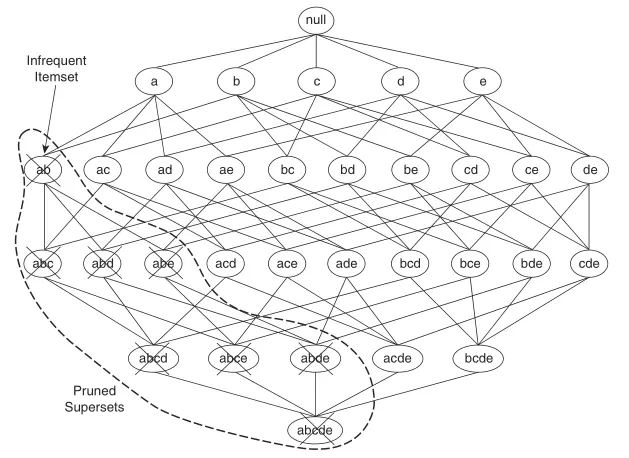
Based on the Apriori principle, if we find that \(\{a, b\}\) is an infrequent itemset, then the entire subgraph of supersets containing \(\{a, b\}\) can be pruned. Thus, the algorithm process for generating frequent itemsets using the Apriori algorithm is as follows:
First, let \(F_k\) denote the set of frequent \(k\)-itemsets and \(C_k\) denote the set of candidate \(k\)-itemsets:
-
The algorithm scans the entire dataset once, calculates the support of each item, and obtains the set \(F_1\) of frequent 1-itemsets.
-
Then, the algorithm generates candidate \(k\)-itemsets using frequent \((k - 1)\)-itemsets, and methods such as \(F_{k - 1} \times F_{k - 1}\) or \(F_{k - 1} \times F_1\) can be used.
-
The algorithm scans the dataset again to complete the support counting for candidate itemsets, and uses the subset function to determine all candidate \(k\)-itemsets in \(C_k\).
-
Calculate the support of candidate itemsets and delete candidate itemsets with support less than the pre-set threshold.
-
When no frequent itemsets are generated, i.e., \(F_k = \emptyset\), the algorithm ends.
After generating frequent itemsets, association rules can be extracted from the given frequent itemsets. Generally, each frequent \(k\)-itemset can generate \(2^k - 2\) association rules. The generated rules need to be pruned based on confidence to meet the pre-set confidence threshold.
Here, we will give another theorem about confidence. Suppose the itemset \(Y\) can be partitioned into two non-empty subsets \(X\) and \(Y - X\), then:
-
If the rule \(X → Y - X\) does not meet the confidence threshold, then the rule \(X' → Y - X'\) must not meet the confidence threshold. Where \(X'\) is a subset of \(X\).
The Apriori algorithm uses a level-wise approach to generate association rules, where each level corresponds to the number of items in the consequent of the rule. Initially, all high-confidence rules with only one item in the second part of the rule are extracted; then, these rules are used to generate new candidate rules.
34.10. Association Rule Practice#
Although association rules ultimately boil down to finding frequent itemsets and calculating confidence, which may sound simple, the process of making the calculation efficient can be rather troublesome. Take the Apriori algorithm as an example. A complete Python implementation would require approximately 200+ lines of code. Therefore, in this experiment, we will not implement it manually.
Next, we use association rule mining to conduct a practical exercise on a sample sales dataset. Here, we use the Apriori algorithm API provided by the mlxtend machine learning algorithm library. This API is implemented exactly according to the paper Fast algorithms for mining association rules in large databases.
First, here is a sample shopping dataset where each list in the two-dimensional list represents the names of items in a single shopping cart.
dataset = [
    ["牛奶", "洋葱", "牛肉", "芸豆", "鸡蛋", "酸奶"],
    ["玉米", "洋葱", "洋葱", "芸豆", "豆腐", "鸡蛋"],
    ["牛奶", "香蕉", "玉米", "芸豆", "酸奶"],
    ["芸豆", "玉米", "香蕉", "牛奶", "鸡蛋"],
    ["香蕉", "牛奶", "鸡蛋", "酸奶"],
    ["牛奶", "苹果", "芸豆", "鸡蛋"],
]
dataset
[['牛奶', '洋葱', '牛肉', '芸豆', '鸡蛋', '酸奶'],
 ['玉米', '洋葱', '洋葱', '芸豆', '豆腐', '鸡蛋'],
 ['牛奶', '香蕉', '玉米', '芸豆', '酸奶'],
 ['芸豆', '玉米', '香蕉', '牛奶', '鸡蛋'],
 ['香蕉', '牛奶', '鸡蛋', '酸奶'],
 ['牛奶', '苹果', '芸豆', '鸡蛋']]
We attempt to generate frequent itemsets through the Apriori
algorithm. Here, we first convert the list data into a
format usable by the Apriori algorithm API via
mlxtend.preprocessing.TransactionEncoder.
mlxtend.preprocessing.TransactionEncoder
is similar to one-hot encoding. It can extract the unique
items in the dataset and convert each shopping cart data
into a boolean representation of equal length. The API
provided by mlxtend is used in a similar way to
scikit-learn.
import pandas as pd
from mlxtend.preprocessing import TransactionEncoder

te = TransactionEncoder()  # 定义模型
te_ary = te.fit_transform(dataset)  # 转换数据集
te_ary
array([[ True,  True,  True, False,  True, False, False,  True, False,
         True],
       [ True, False, False,  True,  True, False,  True, False, False,
         True],
       [False,  True, False,  True,  True, False, False,  True,  True,
        False],
       [False,  True, False,  True,  True, False, False, False,  True,
         True],
       [False,  True, False, False, False, False, False,  True,  True,
         True],
       [False,  True, False, False,  True,  True, False, False, False,
         True]])
Finally, the shopping cart dataset is represented as follows:
df = pd.DataFrame(te_ary, columns=te.columns_)  # 将数组处理为 DataFrame
df
| 洋葱 | 牛奶 | 牛肉 | 玉米 | 芸豆 | 苹果 | 豆腐 | 酸奶 | 香蕉 | 鸡蛋 | |
|---|---|---|---|---|---|---|---|---|---|---|
| 0 | True | True | True | False | True | False | False | True | False | True |
| 1 | True | False | False | True | True | False | True | False | False | True |
| 2 | False | True | False | True | True | False | False | True | True | False |
| 3 | False | True | False | True | True | False | False | False | True | True |
| 4 | False | True | False | False | False | False | False | True | True | True |
| 5 | False | True | False | False | True | True | False | False | False | True |
Next, we can use the
mlxtend.frequent_patterns.apriori
API to generate frequent itemsets. According to the previous
learning, when generating frequent itemsets, it is necessary
to specify the minimum support threshold, and the candidate
sets that meet the threshold will be designated as frequent
itemsets.
from mlxtend.frequent_patterns import apriori

apriori(df, min_support=0.5)  # 最小支持度为 0.5
| support | itemsets | |
|---|---|---|
| 0 | 0.833333 | (1) |
| 1 | 0.500000 | (3) |
| 2 | 0.833333 | (4) |
| 3 | 0.500000 | (7) |
| 4 | 0.500000 | (8) |
| 5 | 0.833333 | (9) |
| 6 | 0.666667 | (1, 4) |
| 7 | 0.500000 | (1, 7) |
| 8 | 0.500000 | (8, 1) |
| 9 | 0.666667 | (1, 9) |
| 10 | 0.500000 | (3, 4) |
| 11 | 0.666667 | (9, 4) |
| 12 | 0.500000 | (1, 4, 9) |
By default,
apriori
returns items as column indices, which is convenient for
generating association rules. For better readability, here
we can set the
use_colnames=True
parameter to convert the indices to the corresponding item
names:
apriori(df, min_support=0.5, use_colnames=True)
| support | itemsets | |
|---|---|---|
| 0 | 0.833333 | (牛奶) |
| 1 | 0.500000 | (玉米) |
| 2 | 0.833333 | (芸豆) |
| 3 | 0.500000 | (酸奶) |
| 4 | 0.500000 | (香蕉) |
| 5 | 0.833333 | (鸡蛋) |
| 6 | 0.666667 | (牛奶, 芸豆) |
| 7 | 0.500000 | (牛奶, 酸奶) |
| 8 | 0.500000 | (牛奶, 香蕉) |
| 9 | 0.666667 | (牛奶, 鸡蛋) |
| 10 | 0.500000 | (芸豆, 玉米) |
| 11 | 0.666667 | (鸡蛋, 芸豆) |
| 12 | 0.500000 | (牛奶, 鸡蛋, 芸豆) |
At this point, if you only want to view the frequent itemsets that contain at least two items, you can achieve this through Pandas selection:
frequent_itemsets = apriori(df, min_support=0.5, use_colnames=True)
frequent_itemsets[
    frequent_itemsets.itemsets.apply(lambda x: len(x)) >= 2
]  # 选择长度 >=2 的频繁项集
| support | itemsets | |
|---|---|---|
| 6 | 0.666667 | (牛奶, 芸豆) |
| 7 | 0.500000 | (牛奶, 酸奶) |
| 8 | 0.500000 | (牛奶, 香蕉) |
| 9 | 0.666667 | (牛奶, 鸡蛋) |
| 10 | 0.500000 | (芸豆, 玉米) |
| 11 | 0.666667 | (鸡蛋, 芸豆) |
| 12 | 0.500000 | (牛奶, 鸡蛋, 芸豆) |
With the frequent itemsets, next we can use
mlxtend.frequent_patterns.association_rules
to generate association rules. At this time, it is necessary
to specify the minimum confidence threshold.
from mlxtend.frequent_patterns import association_rules

association_rules(
    frequent_itemsets, metric="confidence", min_threshold=0.6
)  # 置信度阈值为 0.6
| antecedents | consequents | antecedent support | consequent support | support | confidence | lift | leverage | conviction | zhangs_metric | |
|---|---|---|---|---|---|---|---|---|---|---|
| 0 | (牛奶) | (芸豆) | 0.833333 | 0.833333 | 0.666667 | 0.80 | 0.96 | -0.027778 | 0.833333 | -0.200000 |
| 1 | (芸豆) | (牛奶) | 0.833333 | 0.833333 | 0.666667 | 0.80 | 0.96 | -0.027778 | 0.833333 | -0.200000 |
| 2 | (牛奶) | (酸奶) | 0.833333 | 0.500000 | 0.500000 | 0.60 | 1.20 | 0.083333 | 1.250000 | 1.000000 |
| 3 | (酸奶) | (牛奶) | 0.500000 | 0.833333 | 0.500000 | 1.00 | 1.20 | 0.083333 | inf | 0.333333 |
| 4 | (牛奶) | (香蕉) | 0.833333 | 0.500000 | 0.500000 | 0.60 | 1.20 | 0.083333 | 1.250000 | 1.000000 |
| 5 | (香蕉) | (牛奶) | 0.500000 | 0.833333 | 0.500000 | 1.00 | 1.20 | 0.083333 | inf | 0.333333 |
| 6 | (牛奶) | (鸡蛋) | 0.833333 | 0.833333 | 0.666667 | 0.80 | 0.96 | -0.027778 | 0.833333 | -0.200000 |
| 7 | (鸡蛋) | (牛奶) | 0.833333 | 0.833333 | 0.666667 | 0.80 | 0.96 | -0.027778 | 0.833333 | -0.200000 |
| 8 | (芸豆) | (玉米) | 0.833333 | 0.500000 | 0.500000 | 0.60 | 1.20 | 0.083333 | 1.250000 | 1.000000 |
| 9 | (玉米) | (芸豆) | 0.500000 | 0.833333 | 0.500000 | 1.00 | 1.20 | 0.083333 | inf | 0.333333 |
| 10 | (鸡蛋) | (芸豆) | 0.833333 | 0.833333 | 0.666667 | 0.80 | 0.96 | -0.027778 | 0.833333 | -0.200000 |
| 11 | (芸豆) | (鸡蛋) | 0.833333 | 0.833333 | 0.666667 | 0.80 | 0.96 | -0.027778 | 0.833333 | -0.200000 |
| 12 | (牛奶, 鸡蛋) | (芸豆) | 0.666667 | 0.833333 | 0.500000 | 0.75 | 0.90 | -0.055556 | 0.666667 | -0.250000 |
| 13 | (牛奶, 芸豆) | (鸡蛋) | 0.666667 | 0.833333 | 0.500000 | 0.75 | 0.90 | -0.055556 | 0.666667 | -0.250000 |
| 14 | (鸡蛋, 芸豆) | (牛奶) | 0.666667 | 0.833333 | 0.500000 | 0.75 | 0.90 | -0.055556 | 0.666667 | -0.250000 |
| 15 | (牛奶) | (鸡蛋, 芸豆) | 0.833333 | 0.666667 | 0.500000 | 0.60 | 0.90 | -0.055556 | 0.833333 | -0.400000 |
| 16 | (鸡蛋) | (牛奶, 芸豆) | 0.833333 | 0.666667 | 0.500000 | 0.60 | 0.90 | -0.055556 | 0.833333 | -0.400000 |
| 17 | (芸豆) | (牛奶, 鸡蛋) | 0.833333 | 0.666667 | 0.500000 | 0.60 | 0.90 | -0.055556 | 0.833333 | -0.400000 |
association_rules(
    frequent_itemsets, metric="confidence", min_threshold=0.8
)  # 置信度阈值为 0.8
| antecedents | consequents | antecedent support | consequent support | support | confidence | lift | leverage | conviction | zhangs_metric | |
|---|---|---|---|---|---|---|---|---|---|---|
| 0 | (酸奶) | (牛奶) | 0.5 | 0.833333 | 0.5 | 1.0 | 1.2 | 0.083333 | inf | 0.333333 |
| 1 | (香蕉) | (牛奶) | 0.5 | 0.833333 | 0.5 | 1.0 | 1.2 | 0.083333 | inf | 0.333333 |
| 2 | (玉米) | (芸豆) | 0.5 | 0.833333 | 0.5 | 1.0 | 1.2 | 0.083333 | inf | 0.333333 |
mlxtend uses a DataFrame instead of → to display association rules. Among them:
-
antecedents: Antecedent of the rule -
consequents: Consequent of the rule -
antecedent
                          support
: Support of the antecedent of the rule -
consequent
                          support
: Support of the consequent of the rule -
support: Support of the rule -
confidence: Confidence of the rule -
lift: Lift of the rule, which represents the ratio of the probability of containing the consequent under the condition of containing the antecedent to the overall occurrence probability of the consequent. -
leverage: Leverage of the rule, which indicates how many more times the antecedent and the consequent appear together than expected when they are independently distributed. -
conviction: Conviction of the rule, similar to lift but expressed as a difference.
In the previous content, we did not introduce the concepts of lift, leverage, and conviction. These are actually supplementary rules for evaluation in association rules and are not necessary.
The formula for calculating lift is as follows:
Among them, when the antecedent and the consequent are independently distributed, the value is 1. The larger the lift, the stronger the correlation between the antecedent and the consequent.
The formula for calculating leverage is as follows:
Among them, when the antecedent and the consequent are independently distributed, the value is 0. The larger the leverage, the stronger the correlation between the antecedent and the consequent.
The formula for calculating confidence is as follows:
The larger the confidence value, the stronger the correlation between the antecedent and the consequent.
34.11. Summary#
In this experiment, we introduced the association rule learning method, focused on understanding several concepts involved, and finally practiced the Apriori algorithm using the mlxtend machine learning library. The experiment did not implement the algorithm in pure Python from the principle because the involved algorithm principle is really troublesome. Of course, if you are interested, here are several open-source projects of the Apriori algorithm recommended for you to check the source code for learning. They are: