
33. Comparative Evaluation of Common Clustering Algorithms#
33.1. Introduction#
Previously, nearly ten clustering algorithms with different ideas were explained. The purpose of the last challenge is to explore the clustering effects and required time of different algorithms on datasets with different shapes.
33.2. Key Points#
Adaptability of algorithms to data shapes
-
Algorithm efficiency under the same conditions
33.3. Generate Test Data#
Before the challenge, it is necessary to generate test data
first. We use
make_moons(),
make_circles(), and
make_blobs()
to generate three sets of data.
{exercise-start}
:label: chapter03_09_1
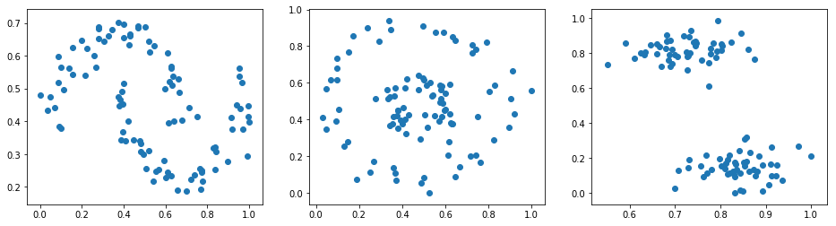
Challenge: Use sklearn to generate three sets of test data and plot scatter plots (subplots concatenated horizontally).
Regulations:
-
For the convenience of subsequent experiments, you need to perform Min-Max normalization on the three sets of test data so that both the horizontal and vertical coordinates are within the range of 0-1.
-
The corresponding parameters for the three methods are as follows:
-
All three sets of data contain 100 samples, and the random number seed is set to 10 for all.
Add 0.1 noise to the moons and circles data.
-
Set the inner and outer circle spacing ratio factor of the circles data to 0.3.
-
The blobs data has 2 clusters, and the cluster standard deviation is set to 1.5.
-
Take the default values for the remaining parameters.
{exercise-end}
Min-Max normalization is also a commonly used method. Its effect is similar to interval scaling, which can scale the values between 0 and 1. Its formula is:
Among them, \(x_{max}\) is the maximum value of the sample data, \(x_{min}\) is the minimum value of the sample data, and \(x_{max}-x_{min}\) is the range.
import numpy as np
from sklearn import datasets
from matplotlib import pyplot as plt

%matplotlib inline

## 代码开始 ### (≈ 7-10 行代码)

## 代码结束 ###
{solution-start} chapter03_09_1
:class: dropdown
import numpy as np
from sklearn import datasets
from matplotlib import pyplot as plt
%matplotlib inline

### Code start ### ((≈ 7-10 lines of code))
moons, _ = datasets.make_moons(n_samples=100, noise=.1, random_state=10)
circles, _ = datasets.make_circles(n_samples=100, noise=.1, factor=.3, random_state=10)
blobs, _ = datasets.make_blobs(n_samples=100, n_features=2, centers=2, cluster_std=1.5, random_state=10)

# Min-Max normalization
moons = (moons - np.min(moons)) / (np.max(moons) - np.min(moons))
circles = (circles - np.min(circles)) / (np.max(circles) - np.min(circles))
blobs = (blobs - np.min(blobs)) / (np.max(blobs) - np.min(blobs))

fig, axes = plt.subplots(nrows=1, ncols=3, figsize=(16, 4))
axes[0].scatter(moons[:, 0], moons[:, 1])
axes[1].scatter(circles[:, 0], circles[:, 1])
axes[2].scatter(blobs[:, 0], blobs[:, 1])
### Code end ###
{solution-end}
Expected output
33.4. Comparison of Clustering Results#
Next, several commonly used clustering methods provided by sklearn are to be selected to test the clustering effects on the above three datasets. These clustering methods are:
-
cluster.KMeans() -
cluster.MiniBatchKMeans() -
cluster.AffinityPropagation() -
cluster.MeanShift() -
cluster.SpectralClustering() -
cluster.AgglomerativeClustering() -
cluster.Birch() -
cluster.DBSCAN()
Exercise 33.1
Challenge: Test the above eight clustering methods on moons, circles, and blobs respectively, and plot the clustering results.
Requirement: No parameters are specified for this challenge. Please make the clustering effect as good as possible based on the content learned previously.
from sklearn import cluster

## 代码开始 ### (> 10 行代码)

## 代码结束 ###
Solution to Exercise 33.1
from sklearn import cluster

### Code start ### (> 10 lines of code)
cluster_names = ['KMeans', 'MiniBatchKMeans', 'AffinityPropagation',
                 'MeanShift', 'SpectralClustering', 'AgglomerativeClustering', 'Birch', 'DBSCAN']

cluster_estimators = [
    cluster.KMeans(n_clusters=2),
    cluster.MiniBatchKMeans(n_clusters=2),
    cluster.AffinityPropagation(),
    cluster.MeanShift(),
    cluster.SpectralClustering(n_clusters=2, metric='nearest_neighbors', n_neighbors=6),
    cluster.AgglomerativeClustering(n_clusters=2),
    cluster.Birch(n_clusters=2, threshold=.1),
    cluster.DBSCAN(eps=.1, min_samples=6, metric='euclidean')
]

for algorithm_name, algorithm in zip(cluster_names, cluster_estimators):

    moons_clusters = algorithm.fit_predict(moons)
    circles_clusters = algorithm.fit_predict(circles)
    blobs_clusters = algorithm.fit_predict(blobs)

    fig, axes = plt.subplots(nrows=1, ncols=3, figsize=(16, 4))
    axes[0].scatter(moons[:, 0],moons[:, 1], c=moons_clusters)
    axes[1].scatter(circles[:, 0],circles[:, 1], c=circles_clusters)
    axes[2].scatter(blobs[:, 0],blobs[:, 1], c=blobs_clusters)
    axes[0].set_ylabel('{}'.format(algorithm_name))
### Code end ###
Expected output
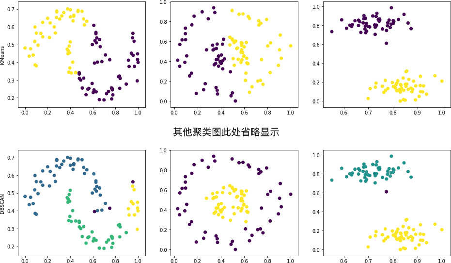
In the above figure, generally, we can only draw conclusions about the clustering effects of the same method on different datasets. Since the clustering effects between different methods depend on specific parameters, we cannot accurately determine which one is better or worse. The results can only be used as a reference.
Next, we want to test the speed comparison of different
methods when executing on datasets of different magnitudes.
This time, we only use
make_blobs()
to generate blob-shaped test data. The function for
generating the test data is as follows:
def create_data(n):
    """
    参数:
    n -- 生成样本数量
    返回:
    blobs_data -- 样本数组
    """
    blobs_data, _ = datasets.make_blobs(
        n_samples=n, n_features=2, centers=2, cluster_std=1.5, random_state=10
    )
    return blobs_data
Exercise 33.2
Challenge: Use
create_data(n)
to generate test data of different scales, calculate the
clustering time of different algorithms, and plot the
corresponding line chart.
Regulations:
-
Generate data scales in sequence: 100, 200, 300, ···, 900, 1000, a total of 10 groups.
-
Except for specifying
n_clusters
                              =
                              2
, use the default parameters of the relevant methods for the rest of the parameters.
Hint: You can record the running time of the algorithm
through the
time
module. For example:
import time

t0 = time.time()
cluster_estimator.fit()
t1 = time.time()
Then
t1 -
                      t0
is the time taken by
cluster_estimator.fit().
import time

## 代码开始 ### (> 10 行代码)

## 代码结束 ###
Solution to Exercise 33.2
import time

### Code start ### (> 10 lines of code)
cluster_names = ['KMeans', 'MiniBatchKMeans', 'AffinityPropagation',
                 'MeanShift', 'SpectralClustering', 'AgglomerativeClustering', 'Birch', 'DBSCAN']

cluster_estimators = [
    cluster.KMeans(n_clusters=2),
    cluster.MiniBatchKMeans(n_clusters=2),
    cluster.AffinityPropagation(),
    cluster.MeanShift(),
    cluster.SpectralClustering(n_clusters=2),
    cluster.AgglomerativeClustering(n_clusters=2),
    cluster.Birch(n_clusters=2),
    cluster.DBSCAN()
]

cluster_t_list = []
for algorithm_name, algorithm in zip(cluster_names, cluster_estimators):
    t_list = []
    for num in [i for i in range(100, 1100, 100)]:
        data = create_data(num) # Generate data
        t0 = time.time()
        moons_clusters = algorithm.fit(data)
        t1 = time.time()
        t_list.append(t1 - t0) # Calculate clustering time
    print("{} fitted & average time:{:4f}".format(algorithm_name, np.mean(t_list)))
    cluster_t_list.append(t_list)

plt.figure(figsize=(12, 6))
for cluster_t, cluster_name in zip(cluster_t_list, cluster_names):
    plt.plot(cluster_t, marker='.', label=cluster_name)
    plt.legend()
### Code end ###
Expected output
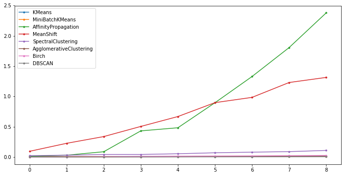
It can be found that Affinity Propagation, Mean Shift, and Spectral Clustering have a relatively fast rising speed of time consumption and are also relatively time-consuming clustering algorithms.