
31. Density Clustering to Mark Abnormal Shared Bicycles#
31.1. Introduction#
This challenge will examine the application of density clustering. We will attempt to use density clustering to visualize the location distribution of shared bicycles and, at the same time, use different parameters to mark the locations of abnormal shared bicycles.
31.2. Key Points#
Determination of DBSCAN parameters
HDBSCAN clustering
Today, shared bicycles can be found everywhere on the streets and alleys, which truly facilitates the short-distance travel of citizens. However, if you are an operator of a shared bicycle company, would you consider such a question: where have all the shared bicycles put into the city by the company gone?
Of course, this question is not to satisfy your curiosity, but to adjust the operation strategy in a timely manner by tracking the distribution of shared bicycles. For example, if the density of bicycles in some locations is too high, then consideration should be given to moving them to areas with low density but demand.
Therefore, in today’s challenge, the density clustering method will be used to track the distribution of shared bicycles.
We obtained a GPS scatter dataset of shared bicycles in a
certain area of Beijing, and the name of this dataset is
challenge-9-bike.csv. First, load and preview this dataset.
wget -nc https://cdn.aibydoing.com/aibydoing/files/challenge-9-bike.csv
import pandas as pd
import numpy as np

df = pd.read_csv("challenge-9-bike.csv")
df.describe()
| lat | lon | |
|---|---|---|
| count | 3000.000000 | 3000.000000 |
| mean | 39.908308 | 116.474630 |
| std | 0.007702 | 0.018098 |
| min | 39.893939 | 116.434264 |
| 25% | 39.902769 | 116.461276 |
| 50% | 39.907888 | 116.477683 |
| 75% | 39.914482 | 116.490274 |
| max | 39.923023 | 116.501467 |
Among them,
lat
is the abbreviation of latitude, representing latitude, and
lon
is the abbreviation of longitude, representing longitude.
Thus, we can use Matplotlib to plot the distribution of
shared bicycles in this area.
from matplotlib import pyplot as plt

%matplotlib inline

plt.figure(figsize=(15, 8))
plt.scatter(df["lat"], df["lon"], alpha=0.6)
<matplotlib.collections.PathCollection at 0x121cb4ac0>

Next, we try to use the DBSCAN density clustering algorithm to cluster the shared bicycles and see the distribution of high-density areas of shared bicycles. (It may not work, but it has no impact on the challenge)
According to the experiment in the previous section, the two
key parameters of the DBSCAN algorithm are
eps
and the density threshold
MinPts. So, what are the appropriate values for these two
parameters?
Exercise 31.1
Challenge: Use the DBSCAN algorithm to complete the
density clustering of the GPS scatter data of shared
bicycles, and determine the
eps
and
min_samples
parameters.
Regulation: Assume that there are 10 vehicles within a radius of 100 meters as a high-density area.
Hint: The challenge takes the change in latitude as a reference. Roughly estimate that a 1-degree change in latitude corresponds to a ground distance of 100 km in this area.
from sklearn.cluster import DBSCAN

## 代码开始 ### (≈ 2 行代码)

## 代码结束 ###
dbscan_c  # 输出聚类标签
Run the test
np.mean(dbscan_c)
Expected output
6.977333333333333
Exercise 31.2
Challenge: For the data after clustering above, redraw the scatter plot as required.
Specification: The unclustered outliers are presented as
blue data points with
alpha=0.1, and the clustered data is presented by category with
cmap='viridis'.
## 代码开始 ### (≈ 4~8 行代码)
plt.figure(figsize=(15, 8))
## 代码结束 ###
Expected output
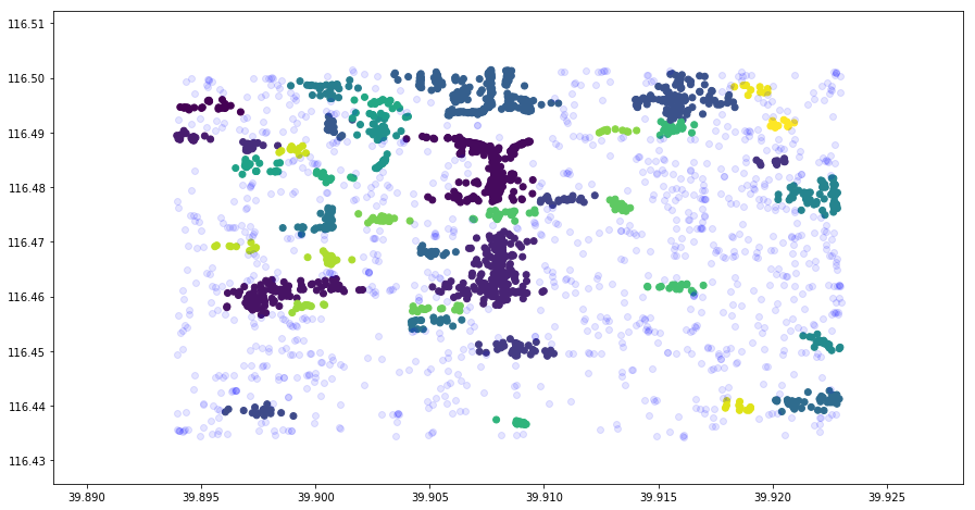
It can be seen from the above figure the distribution of bike density in different areas.
The HDBSCAN algorithm often does more than just perform clustering. Due to its inherent characteristics, it is often used to identify outliers as well. In this experiment, we can also identify shared bikes with abnormal locations by adjusting the parameters.
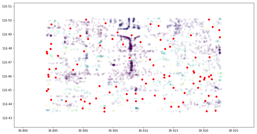
Exercise 31.3
Challenge: For the data after clustering, plot the outliers (not meeting the condition of having 2 shared bikes within a radius of 100 meters) on a scatter plot.
Requirement: The unclustered boundary points are
presented as red data points, and the clustered data is
presented by category with
alpha
                          =
                          0.1
and
cmap='viridis'.
## 代码开始 ### (≈ 6~10 行代码)
plt.figure(figsize=(15, 8))
## 代码结束 ###
Expected output
This challenge mainly focuses on understanding how to quickly determine the initial parameters of DBSCAN and the method of using this algorithm to mark outliers. If you are interested, you can also try using HDBSCAN for clustering by yourself and compare the clustering effects of the two. Of course, before that, you need to install the hdbscan module using the method in the experiment.