Pro Membership

Pro Membership is a membership plan created by the author to maintain and update this tutorial. You can get more benefits and services, click to view details.

27. Implementation and Application of Hierarchical Clustering Method

27.1. Introduction

In the previous experiment, we learned about partitioning clustering methods, especially the two excellent clustering algorithms, K-Means and K-Means++. This experiment will introduce a completely different type of clustering method, namely hierarchical clustering. Hierarchical clustering can help effectively avoid the trouble of having to specify the number of clusters in advance when using partitioning clustering. In addition, it can also be applied in some specific scenarios.

27.2. Key Points

• Overview of Hierarchical Clustering Method

• Bottom-up Hierarchical Clustering Method

• Top-down Hierarchical Clustering Method

• BIRCH Clustering Algorithm

• PCA (Principal Component Analysis)

27.3. Overview of Hierarchical Clustering Method

In the content of the previous class, we learned about partitioning clustering methods and focused on introducing the K-Means algorithm among them. The K-Means algorithm can be said to be one of the clustering algorithms with very wide applications and it is very useful. However, after you have used this algorithm, you will find a rather “headache-inducing” problem, that is, we need to manually specify the value of K, which is the number of clusters.

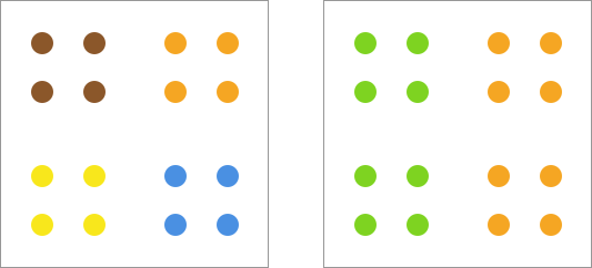
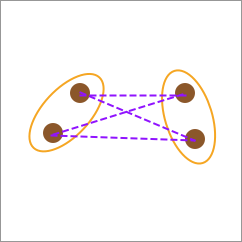
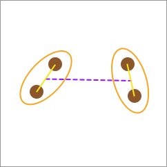
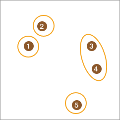
Determining the number of clusters in advance may seem like a minor matter, but it can be quite troublesome in many cases because we may not know how many clusters the dataset should be grouped into before clustering. For example, in the following schematic diagram, it seems reasonable to group it into either 2 or 4 clusters.

One of the biggest differences between the hierarchical clustering method we are going to learn today and partitioning clustering is that we don’t need to specify the number of clusters in advance. This sounds very attractive. How exactly is it achieved?

Simply put, the characteristic of the hierarchical clustering method is to generate a tree with a hierarchical structure by calculating the similarity between the elements of the dataset. First, it should be emphasized here that this “hierarchical tree” is completely different from the “decision tree” learned in the second week’s course and don’t confuse them.

Meanwhile, when we use the hierarchical clustering method, it can be divided into two cases according to the way of creating the tree:

• Bottom-up hierarchical clustering method: The process of this method is called “agglomerative”, that is, each element in the dataset is regarded as a category, and then iteratively merged into larger categories until a certain termination condition is met.

• Top-down hierarchical clustering method: The process of this method is called “divisive”, which is the reverse process of agglomeration. First, the dataset is regarded as a category, and then recursively divided into multiple smaller subcategories until a certain termination condition is met.

27.4. Bottom-up hierarchical clustering method

The bottom-up hierarchical clustering method is also the Agglomerative Clustering algorithm. The main feature of this algorithm is that we use the idea of “bottom-up” clustering to help samples that are close in distance be placed in the same category. Specifically, the main steps of this method are as follows:

For the dataset \(D\), \(D = (x_1, x_2, \cdots, x_n)\):

1. Label each sample in the dataset as a single class. That is, initially, the classes (\(C\)) contained in \(D\) are \(C = (c_1, c_2, \cdots, c_n)\).

2. Calculate and find the two closest classes in \(C\) and merge them into one class.

3. Keep merging in sequence until only one list remains, thus building a complete hierarchical tree.

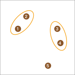
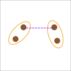
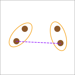
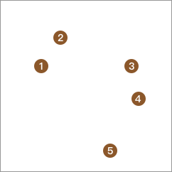
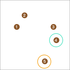
We use the following figure to demonstrate the process of the bottom-up hierarchical clustering method. First, there are 5 sample points on the plane, and we divide each sample point into a separate class.

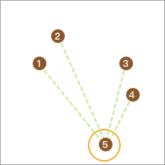
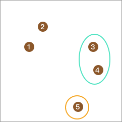
Next, we can calculate the distances between elements and merge the ones with the closest distance into one class. As a result, the total number of classes becomes 3.

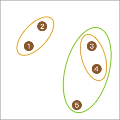
Repeat the above steps, and the total number of classes becomes 2.

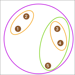
Finally, it is merged into one class and the clustering terminates.

When we transform the above clustering process into a hierarchical tree, it becomes:

After watching the above demonstration process, you will find that the “bottom-up hierarchical clustering method” is actually so simple.

27.5. Distance Calculation Methods

Although the clustering process seems simple, I wonder if you have realized a problem: when a category contains multiple elements, how is the distance between categories determined?

That is to say, in the above demonstration process, why is 5 classified into the category composed of <3, 4> instead of the category composed of <1, 2>? Or rather, why don’t we first merge <1, 2> and <3, 4>, and finally merge 5?

This involves the distance calculation method in the Agglomerative clustering process. Briefly speaking, we generally have 3 different distance calculation methods:

27.6. Single-linkage

The calculation method of single-linkage is to use the distance between the closest elements between two categories as the distance between the two categories.

27.7. Complete-linkage

The calculation method of complete-linkage is to use the distance between the farthest elements between two categories as the distance between the two categories.

27.8. Average-linkage

The calculation method of average-linkage is to calculate the distances between each pair of elements between two categories in turn, and finally obtain the average value as the distance between the two categories.

27.9. Center-linkage

Although average-linkage seems more reasonable, the computational cost of calculating the distances between each pair of elements is often extremely large. Sometimes, the center-linkage calculation method can also be used. That is, first calculate the category centers, and then use the line connecting the centers as the distance between the two categories.

In summary, among the above four distance calculation methods, the “average-linkage” and “center-linkage” methods are generally commonly used because both “single-linkage” and “complete-linkage” are relatively extreme and are prone to interference caused by noise points and unevenly distributed data.

27.10. Agglomerative Clustering Python Implementation

Next, we will attempt to implement the bottom-up hierarchical clustering algorithm in Python.

Generate a set of sample data randomly through the make_blobs method, and make the sample data show a trend of two types of data. Here, we set the random number seed random_state = 10 to ensure that your results are consistent with the experimental results.

from sklearn import datasets

data = datasets.make_blobs(10, n_features=2, centers=2, random_state=10)
data

(array([[  6.04774884, -10.30504657],
        [  2.90159483,   5.42121526],
        [  4.1575017 ,   3.89627276],
        [  1.53636249,   5.11121453],
        [  3.88101257,  -9.59334486],
        [  1.70789903,   6.00435173],
        [  5.69192445,  -9.47641249],
        [  5.4307043 ,  -9.75956122],
        [  5.85943906,  -8.38192364],
        [  0.69523642,   3.23270535]]),
 array([0, 1, 1, 1, 0, 1, 0, 0, 0, 1]))

Using Matplotlib to plot the results of the sample data, it can be seen that the data indeed shows a trend of two categories. The result of data[1] is the preset category when generating the data. Of course, in the following clustering process, we do not know the preset category of the data.

from matplotlib import pyplot as plt

%matplotlib inline

plt.scatter(data[0][:, 0], data[0][:, 1], c=data[1], s=60)

<matplotlib.collections.PathCollection at 0x15becbca0>

First, we implement the function to calculate the Euclidean distance:

import numpy as np


def euclidean_distance(a, b):
    """
    参数:
    a -- 数组 a
    b -- 数组 b

    返回:
    dist -- a, b 间欧式距离
    """
    # 欧式距离
    x = float(a[0]) - float(b[0])
    x = x * x
    y = float(a[1]) - float(b[1])
    y = y * y
    dist = round(np.sqrt(x + y), 2)
    return dist

Then, implement the Agglomerative clustering function, using the centroid linkage method here. To more specifically demonstrate the process of hierarchical clustering, some redundant print() functions are added to the function here.

def agglomerative_clustering(data):
    # Agglomerative 聚类计算过程

    while len(data) > 1:
        print("☞ 第 {} 次迭代\n".format(10 - len(data) + 1))
        min_distance = float("inf")  # 设定初始距离为无穷大
        for i in range(len(data)):
            print("---")
            for j in range(i + 1, len(data)):
                distance = euclidean_distance(data[i], data[j])
                print("计算 {} 与 {} 距离为 {}".format(data[i], data[j], distance))
                if distance < min_distance:
                    min_distance = distance
                    min_ij = (i, j)
        i, j = min_ij  # 最近数据点序号
        data1 = data[i]
        data2 = data[j]
        data = np.delete(data, j, 0)  # 删除原数据
        data = np.delete(data, i, 0)  # 删除原数据
        b = np.atleast_2d(
            [(data1[0] + data2[0]) / 2, (data1[1] + data2[1]) / 2]
        )  # 计算两点新中心
        data = np.concatenate((data, b), axis=0)  # 将新数据点添加到迭代过程
        print("\n最近距离:{} & {} = {}, 合并后中心:{}\n".format(data1, data2, min_distance, b))

    return data

agglomerative_clustering(data[0])

☞ 第 1 次迭代

---
计算 [  6.04774884 -10.30504657] 与 [2.90159483 5.42121526] 距离为 16.04
计算 [  6.04774884 -10.30504657] 与 [4.1575017  3.89627276] 距离为 14.33
计算 [  6.04774884 -10.30504657] 与 [1.53636249 5.11121453] 距离为 16.06
计算 [  6.04774884 -10.30504657] 与 [ 3.88101257 -9.59334486] 距离为 2.28
计算 [  6.04774884 -10.30504657] 与 [1.70789903 6.00435173] 距离为 16.88
计算 [  6.04774884 -10.30504657] 与 [ 5.69192445 -9.47641249] 距离为 0.9
计算 [  6.04774884 -10.30504657] 与 [ 5.4307043  -9.75956122] 距离为 0.82
计算 [  6.04774884 -10.30504657] 与 [ 5.85943906 -8.38192364] 距离为 1.93
计算 [  6.04774884 -10.30504657] 与 [0.69523642 3.23270535] 距离为 14.56
---
计算 [2.90159483 5.42121526] 与 [4.1575017  3.89627276] 距离为 1.98
计算 [2.90159483 5.42121526] 与 [1.53636249 5.11121453] 距离为 1.4
计算 [2.90159483 5.42121526] 与 [ 3.88101257 -9.59334486] 距离为 15.05
计算 [2.90159483 5.42121526] 与 [1.70789903 6.00435173] 距离为 1.33
计算 [2.90159483 5.42121526] 与 [ 5.69192445 -9.47641249] 距离为 15.16
计算 [2.90159483 5.42121526] 与 [ 5.4307043  -9.75956122] 距离为 15.39
计算 [2.90159483 5.42121526] 与 [ 5.85943906 -8.38192364] 距离为 14.12
计算 [2.90159483 5.42121526] 与 [0.69523642 3.23270535] 距离为 3.11
---
计算 [4.1575017  3.89627276] 与 [1.53636249 5.11121453] 距离为 2.89
计算 [4.1575017  3.89627276] 与 [ 3.88101257 -9.59334486] 距离为 13.49
计算 [4.1575017  3.89627276] 与 [1.70789903 6.00435173] 距离为 3.23
计算 [4.1575017  3.89627276] 与 [ 5.69192445 -9.47641249] 距离为 13.46
计算 [4.1575017  3.89627276] 与 [ 5.4307043  -9.75956122] 距离为 13.72
计算 [4.1575017  3.89627276] 与 [ 5.85943906 -8.38192364] 距离为 12.4
计算 [4.1575017  3.89627276] 与 [0.69523642 3.23270535] 距离为 3.53
---
计算 [1.53636249 5.11121453] 与 [ 3.88101257 -9.59334486] 距离为 14.89
计算 [1.53636249 5.11121453] 与 [1.70789903 6.00435173] 距离为 0.91
计算 [1.53636249 5.11121453] 与 [ 5.69192445 -9.47641249] 距离为 15.17
计算 [1.53636249 5.11121453] 与 [ 5.4307043  -9.75956122] 距离为 15.37
计算 [1.53636249 5.11121453] 与 [ 5.85943906 -8.38192364] 距离为 14.17
计算 [1.53636249 5.11121453] 与 [0.69523642 3.23270535] 距离为 2.06
---
计算 [ 3.88101257 -9.59334486] 与 [1.70789903 6.00435173] 距离为 15.75
计算 [ 3.88101257 -9.59334486] 与 [ 5.69192445 -9.47641249] 距离为 1.81
计算 [ 3.88101257 -9.59334486] 与 [ 5.4307043  -9.75956122] 距离为 1.56
计算 [ 3.88101257 -9.59334486] 与 [ 5.85943906 -8.38192364] 距离为 2.32
计算 [ 3.88101257 -9.59334486] 与 [0.69523642 3.23270535] 距离为 13.22
---
计算 [1.70789903 6.00435173] 与 [ 5.69192445 -9.47641249] 距离为 15.99
计算 [1.70789903 6.00435173] 与 [ 5.4307043  -9.75956122] 距离为 16.2
计算 [1.70789903 6.00435173] 与 [ 5.85943906 -8.38192364] 距离为 14.97
计算 [1.70789903 6.00435173] 与 [0.69523642 3.23270535] 距离为 2.95
---
计算 [ 5.69192445 -9.47641249] 与 [ 5.4307043  -9.75956122] 距离为 0.39
计算 [ 5.69192445 -9.47641249] 与 [ 5.85943906 -8.38192364] 距离为 1.11
计算 [ 5.69192445 -9.47641249] 与 [0.69523642 3.23270535] 距离为 13.66
---
计算 [ 5.4307043  -9.75956122] 与 [ 5.85943906 -8.38192364] 距离为 1.44
计算 [ 5.4307043  -9.75956122] 与 [0.69523642 3.23270535] 距离为 13.83
---
计算 [ 5.85943906 -8.38192364] 与 [0.69523642 3.23270535] 距离为 12.71
---

最近距离:[ 5.69192445 -9.47641249] & [ 5.4307043  -9.75956122] = 0.39, 合并后中心:[[ 5.56131437 -9.61798686]]

☞ 第 2 次迭代

---
计算 [  6.04774884 -10.30504657] 与 [2.90159483 5.42121526] 距离为 16.04
计算 [  6.04774884 -10.30504657] 与 [4.1575017  3.89627276] 距离为 14.33
计算 [  6.04774884 -10.30504657] 与 [1.53636249 5.11121453] 距离为 16.06
计算 [  6.04774884 -10.30504657] 与 [ 3.88101257 -9.59334486] 距离为 2.28
计算 [  6.04774884 -10.30504657] 与 [1.70789903 6.00435173] 距离为 16.88
计算 [  6.04774884 -10.30504657] 与 [ 5.85943906 -8.38192364] 距离为 1.93
计算 [  6.04774884 -10.30504657] 与 [0.69523642 3.23270535] 距离为 14.56
计算 [  6.04774884 -10.30504657] 与 [ 5.56131437 -9.61798686] 距离为 0.84
---
计算 [2.90159483 5.42121526] 与 [4.1575017  3.89627276] 距离为 1.98
计算 [2.90159483 5.42121526] 与 [1.53636249 5.11121453] 距离为 1.4
计算 [2.90159483 5.42121526] 与 [ 3.88101257 -9.59334486] 距离为 15.05
计算 [2.90159483 5.42121526] 与 [1.70789903 6.00435173] 距离为 1.33
计算 [2.90159483 5.42121526] 与 [ 5.85943906 -8.38192364] 距离为 14.12
计算 [2.90159483 5.42121526] 与 [0.69523642 3.23270535] 距离为 3.11
计算 [2.90159483 5.42121526] 与 [ 5.56131437 -9.61798686] 距离为 15.27
---
计算 [4.1575017  3.89627276] 与 [1.53636249 5.11121453] 距离为 2.89
计算 [4.1575017  3.89627276] 与 [ 3.88101257 -9.59334486] 距离为 13.49
计算 [4.1575017  3.89627276] 与 [1.70789903 6.00435173] 距离为 3.23
计算 [4.1575017  3.89627276] 与 [ 5.85943906 -8.38192364] 距离为 12.4
计算 [4.1575017  3.89627276] 与 [0.69523642 3.23270535] 距离为 3.53
计算 [4.1575017  3.89627276] 与 [ 5.56131437 -9.61798686] 距离为 13.59
---
计算 [1.53636249 5.11121453] 与 [ 3.88101257 -9.59334486] 距离为 14.89
计算 [1.53636249 5.11121453] 与 [1.70789903 6.00435173] 距离为 0.91
计算 [1.53636249 5.11121453] 与 [ 5.85943906 -8.38192364] 距离为 14.17
计算 [1.53636249 5.11121453] 与 [0.69523642 3.23270535] 距离为 2.06
计算 [1.53636249 5.11121453] 与 [ 5.56131437 -9.61798686] 距离为 15.27
---
计算 [ 3.88101257 -9.59334486] 与 [1.70789903 6.00435173] 距离为 15.75
计算 [ 3.88101257 -9.59334486] 与 [ 5.85943906 -8.38192364] 距离为 2.32
计算 [ 3.88101257 -9.59334486] 与 [0.69523642 3.23270535] 距离为 13.22
计算 [ 3.88101257 -9.59334486] 与 [ 5.56131437 -9.61798686] 距离为 1.68
---
计算 [1.70789903 6.00435173] 与 [ 5.85943906 -8.38192364] 距离为 14.97
计算 [1.70789903 6.00435173] 与 [0.69523642 3.23270535] 距离为 2.95
计算 [1.70789903 6.00435173] 与 [ 5.56131437 -9.61798686] 距离为 16.09
---
计算 [ 5.85943906 -8.38192364] 与 [0.69523642 3.23270535] 距离为 12.71
计算 [ 5.85943906 -8.38192364] 与 [ 5.56131437 -9.61798686] 距离为 1.27
---
计算 [0.69523642 3.23270535] 与 [ 5.56131437 -9.61798686] 距离为 13.74
---

最近距离:[  6.04774884 -10.30504657] & [ 5.56131437 -9.61798686] = 0.84, 合并后中心:[[ 5.80453161 -9.96151671]]

☞ 第 3 次迭代

---
计算 [2.90159483 5.42121526] 与 [4.1575017  3.89627276] 距离为 1.98
计算 [2.90159483 5.42121526] 与 [1.53636249 5.11121453] 距离为 1.4
计算 [2.90159483 5.42121526] 与 [ 3.88101257 -9.59334486] 距离为 15.05
计算 [2.90159483 5.42121526] 与 [1.70789903 6.00435173] 距离为 1.33
计算 [2.90159483 5.42121526] 与 [ 5.85943906 -8.38192364] 距离为 14.12
计算 [2.90159483 5.42121526] 与 [0.69523642 3.23270535] 距离为 3.11
计算 [2.90159483 5.42121526] 与 [ 5.80453161 -9.96151671] 距离为 15.65
---
计算 [4.1575017  3.89627276] 与 [1.53636249 5.11121453] 距离为 2.89
计算 [4.1575017  3.89627276] 与 [ 3.88101257 -9.59334486] 距离为 13.49
计算 [4.1575017  3.89627276] 与 [1.70789903 6.00435173] 距离为 3.23
计算 [4.1575017  3.89627276] 与 [ 5.85943906 -8.38192364] 距离为 12.4
计算 [4.1575017  3.89627276] 与 [0.69523642 3.23270535] 距离为 3.53
计算 [4.1575017  3.89627276] 与 [ 5.80453161 -9.96151671] 距离为 13.96
---
计算 [1.53636249 5.11121453] 与 [ 3.88101257 -9.59334486] 距离为 14.89
计算 [1.53636249 5.11121453] 与 [1.70789903 6.00435173] 距离为 0.91
计算 [1.53636249 5.11121453] 与 [ 5.85943906 -8.38192364] 距离为 14.17
计算 [1.53636249 5.11121453] 与 [0.69523642 3.23270535] 距离为 2.06
计算 [1.53636249 5.11121453] 与 [ 5.80453161 -9.96151671] 距离为 15.67
---
计算 [ 3.88101257 -9.59334486] 与 [1.70789903 6.00435173] 距离为 15.75
计算 [ 3.88101257 -9.59334486] 与 [ 5.85943906 -8.38192364] 距离为 2.32
计算 [ 3.88101257 -9.59334486] 与 [0.69523642 3.23270535] 距离为 13.22
计算 [ 3.88101257 -9.59334486] 与 [ 5.80453161 -9.96151671] 距离为 1.96
---
计算 [1.70789903 6.00435173] 与 [ 5.85943906 -8.38192364] 距离为 14.97
计算 [1.70789903 6.00435173] 与 [0.69523642 3.23270535] 距离为 2.95
计算 [1.70789903 6.00435173] 与 [ 5.80453161 -9.96151671] 距离为 16.48
---
计算 [ 5.85943906 -8.38192364] 与 [0.69523642 3.23270535] 距离为 12.71
计算 [ 5.85943906 -8.38192364] 与 [ 5.80453161 -9.96151671] 距离为 1.58
---
计算 [0.69523642 3.23270535] 与 [ 5.80453161 -9.96151671] 距离为 14.15
---

最近距离:[1.53636249 5.11121453] & [1.70789903 6.00435173] = 0.91, 合并后中心:[[1.62213076 5.55778313]]

☞ 第 4 次迭代

---
计算 [2.90159483 5.42121526] 与 [4.1575017  3.89627276] 距离为 1.98
计算 [2.90159483 5.42121526] 与 [ 3.88101257 -9.59334486] 距离为 15.05
计算 [2.90159483 5.42121526] 与 [ 5.85943906 -8.38192364] 距离为 14.12
计算 [2.90159483 5.42121526] 与 [0.69523642 3.23270535] 距离为 3.11
计算 [2.90159483 5.42121526] 与 [ 5.80453161 -9.96151671] 距离为 15.65
计算 [2.90159483 5.42121526] 与 [1.62213076 5.55778313] 距离为 1.29
---
计算 [4.1575017  3.89627276] 与 [ 3.88101257 -9.59334486] 距离为 13.49
计算 [4.1575017  3.89627276] 与 [ 5.85943906 -8.38192364] 距离为 12.4
计算 [4.1575017  3.89627276] 与 [0.69523642 3.23270535] 距离为 3.53
计算 [4.1575017  3.89627276] 与 [ 5.80453161 -9.96151671] 距离为 13.96
计算 [4.1575017  3.89627276] 与 [1.62213076 5.55778313] 距离为 3.03
---
计算 [ 3.88101257 -9.59334486] 与 [ 5.85943906 -8.38192364] 距离为 2.32
计算 [ 3.88101257 -9.59334486] 与 [0.69523642 3.23270535] 距离为 13.22
计算 [ 3.88101257 -9.59334486] 与 [ 5.80453161 -9.96151671] 距离为 1.96
计算 [ 3.88101257 -9.59334486] 与 [1.62213076 5.55778313] 距离为 15.32
---
计算 [ 5.85943906 -8.38192364] 与 [0.69523642 3.23270535] 距离为 12.71
计算 [ 5.85943906 -8.38192364] 与 [ 5.80453161 -9.96151671] 距离为 1.58
计算 [ 5.85943906 -8.38192364] 与 [1.62213076 5.55778313] 距离为 14.57
---
计算 [0.69523642 3.23270535] 与 [ 5.80453161 -9.96151671] 距离为 14.15
计算 [0.69523642 3.23270535] 与 [1.62213076 5.55778313] 距离为 2.5
---
计算 [ 5.80453161 -9.96151671] 与 [1.62213076 5.55778313] 距离为 16.07
---

最近距离:[2.90159483 5.42121526] & [1.62213076 5.55778313] = 1.29, 合并后中心:[[2.26186279 5.4894992 ]]

☞ 第 5 次迭代

---
计算 [4.1575017  3.89627276] 与 [ 3.88101257 -9.59334486] 距离为 13.49
计算 [4.1575017  3.89627276] 与 [ 5.85943906 -8.38192364] 距离为 12.4
计算 [4.1575017  3.89627276] 与 [0.69523642 3.23270535] 距离为 3.53
计算 [4.1575017  3.89627276] 与 [ 5.80453161 -9.96151671] 距离为 13.96
计算 [4.1575017  3.89627276] 与 [2.26186279 5.4894992 ] 距离为 2.48
---
计算 [ 3.88101257 -9.59334486] 与 [ 5.85943906 -8.38192364] 距离为 2.32
计算 [ 3.88101257 -9.59334486] 与 [0.69523642 3.23270535] 距离为 13.22
计算 [ 3.88101257 -9.59334486] 与 [ 5.80453161 -9.96151671] 距离为 1.96
计算 [ 3.88101257 -9.59334486] 与 [2.26186279 5.4894992 ] 距离为 15.17
---
计算 [ 5.85943906 -8.38192364] 与 [0.69523642 3.23270535] 距离为 12.71
计算 [ 5.85943906 -8.38192364] 与 [ 5.80453161 -9.96151671] 距离为 1.58
计算 [ 5.85943906 -8.38192364] 与 [2.26186279 5.4894992 ] 距离为 14.33
---
计算 [0.69523642 3.23270535] 与 [ 5.80453161 -9.96151671] 距离为 14.15
计算 [0.69523642 3.23270535] 与 [2.26186279 5.4894992 ] 距离为 2.75
---
计算 [ 5.80453161 -9.96151671] 与 [2.26186279 5.4894992 ] 距离为 15.85
---

最近距离:[ 5.85943906 -8.38192364] & [ 5.80453161 -9.96151671] = 1.58, 合并后中心:[[ 5.83198533 -9.17172018]]

☞ 第 6 次迭代

---
计算 [4.1575017  3.89627276] 与 [ 3.88101257 -9.59334486] 距离为 13.49
计算 [4.1575017  3.89627276] 与 [0.69523642 3.23270535] 距离为 3.53
计算 [4.1575017  3.89627276] 与 [2.26186279 5.4894992 ] 距离为 2.48
计算 [4.1575017  3.89627276] 与 [ 5.83198533 -9.17172018] 距离为 13.17
---
计算 [ 3.88101257 -9.59334486] 与 [0.69523642 3.23270535] 距离为 13.22
计算 [ 3.88101257 -9.59334486] 与 [2.26186279 5.4894992 ] 距离为 15.17
计算 [ 3.88101257 -9.59334486] 与 [ 5.83198533 -9.17172018] 距离为 2.0
---
计算 [0.69523642 3.23270535] 与 [2.26186279 5.4894992 ] 距离为 2.75
计算 [0.69523642 3.23270535] 与 [ 5.83198533 -9.17172018] 距离为 13.43
---
计算 [2.26186279 5.4894992 ] 与 [ 5.83198533 -9.17172018] 距离为 15.09
---

最近距离:[ 3.88101257 -9.59334486] & [ 5.83198533 -9.17172018] = 2.0, 合并后中心:[[ 4.85649895 -9.38253252]]

☞ 第 7 次迭代

---
计算 [4.1575017  3.89627276] 与 [0.69523642 3.23270535] 距离为 3.53
计算 [4.1575017  3.89627276] 与 [2.26186279 5.4894992 ] 距离为 2.48
计算 [4.1575017  3.89627276] 与 [ 4.85649895 -9.38253252] 距离为 13.3
---
计算 [0.69523642 3.23270535] 与 [2.26186279 5.4894992 ] 距离为 2.75
计算 [0.69523642 3.23270535] 与 [ 4.85649895 -9.38253252] 距离为 13.28
---
计算 [2.26186279 5.4894992 ] 与 [ 4.85649895 -9.38253252] 距离为 15.1
---

最近距离:[4.1575017  3.89627276] & [2.26186279 5.4894992 ] = 2.48, 合并后中心:[[3.20968225 4.69288598]]

☞ 第 8 次迭代

---
计算 [0.69523642 3.23270535] 与 [ 4.85649895 -9.38253252] 距离为 13.28
计算 [0.69523642 3.23270535] 与 [3.20968225 4.69288598] 距离为 2.91
---
计算 [ 4.85649895 -9.38253252] 与 [3.20968225 4.69288598] 距离为 14.17
---

最近距离:[0.69523642 3.23270535] & [3.20968225 4.69288598] = 2.91, 合并后中心:[[1.95245933 3.96279567]]

☞ 第 9 次迭代

---
计算 [ 4.85649895 -9.38253252] 与 [1.95245933 3.96279567] 距离为 13.66
---

最近距离:[ 4.85649895 -9.38253252] & [1.95245933 3.96279567] = 13.66, 合并后中心:[[ 3.40447914 -2.70986843]]

array([[ 3.40447914, -2.70986843]])

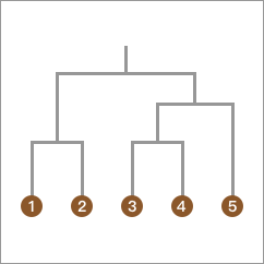
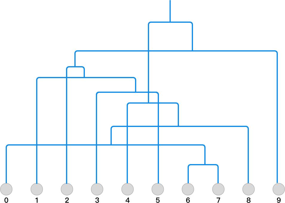
Through the above calculation process, you should be able to clearly see the complete process of Agglomerative clustering. We number each row of the data array from 0 to 9 in sequence, and draw the calculation process into a binary tree structure of hierarchical clustering as follows:

After establishing the tree structure, if we want to select the category 2, we can draw a horizontal line from the top. Then, by following the network to the leaf nodes, we can find their corresponding categories. As shown in the following figure:

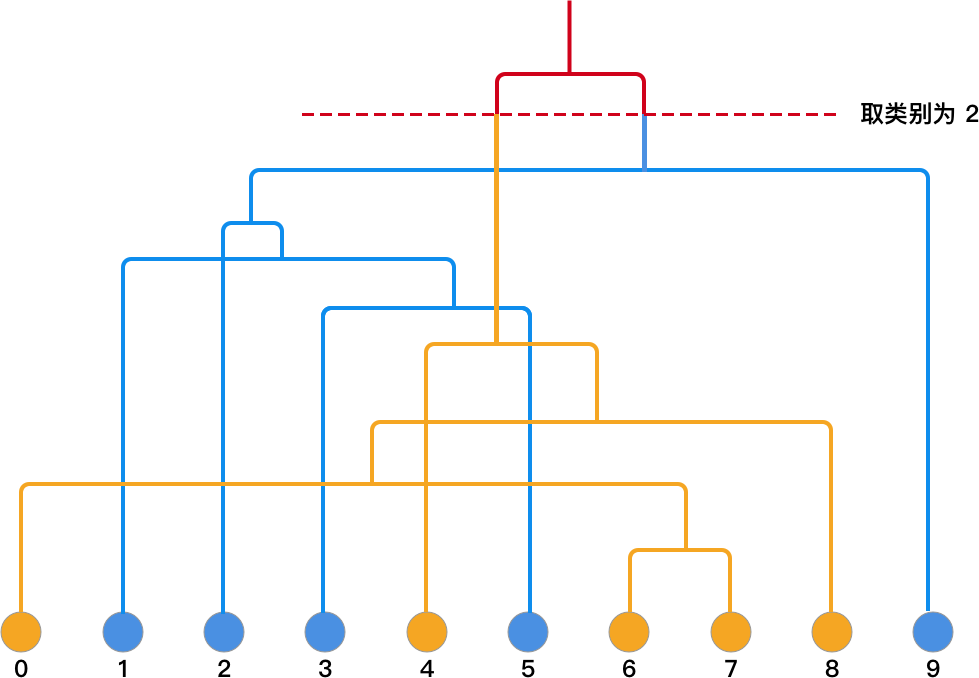
If you look at the preset categories of data, you will find that the final clustering result is exactly the same as data[1] = [0, 1, 1, 1, 0, 1, 0, 0, 0, 1].

So far, we have completely implemented the bottom-up hierarchical clustering method.

27.11. Completing Agglomerative Clustering with scikit-learn

scikit-learn also provides a class for Agglomerative clustering, and the corresponding parameter explanations are as follows:

sklearn.cluster.AgglomerativeClustering(n_clusters=2, metric='euclidean', memory=None, connectivity=None, compute_full_tree='auto', linkage='ward', pooling_func=<function mean>)

Among them:

• n_clusters: Indicates the number of categories to be found finally, such as 2 categories above.

• metric: Options include euclidean (Euclidean distance), l1 (L1 norm), l2 (L2 norm), manhattan (Manhattan distance), etc.

• linkage: Linkage methods: Options include ward (single linkage), complete (complete linkage), average (average linkage).

The experiment also uses the above dataset to complete model construction and clustering:

from sklearn.cluster import AgglomerativeClustering

model = AgglomerativeClustering(n_clusters=2, metric="euclidean", linkage="average")
model.fit_predict(data[0])

array([1, 0, 0, 0, 1, 0, 1, 1, 1, 0])

It can be seen that the final clustering structure is the same as ours above. (The reversal of 1, 0 indicating categories has no impact.)

27.12. Top-Down Hierarchical Clustering Method

In addition to the bottom-up hierarchical clustering method mentioned above, there is also a type of top-down hierarchical clustering method. The calculation process of this method is exactly the opposite of the previous one, but the process is much more complex. Generally speaking, we first classify all the data into one category, and then gradually divide it into smaller categories. There are two common forms of the division method here:

27.13. Using the K-Means Algorithm for Division

First, let’s talk about the division method using the K-Means algorithm:

1. Classify the dataset \(D\) into a single category \(C\) as the top layer.

2. Use the K-Means algorithm to divide \(C\) into two sub-categories to form a sub-layer;

3. Recursively use the K-Means algorithm to continue dividing the sub-layer until the termination condition is met.

Similarly, we can use a schematic diagram to demonstrate the process of this clustering algorithm.

First, all the data is in one category:

Then, use the K-Means algorithm to cluster it into two classes.

Immediately afterwards, use the K-Means algorithm to cluster each subclass into two classes respectively.

Finally, until all the data are each in one category, that is, the segmentation is completed.

The process of using the K-Means algorithm for top-down hierarchical clustering also belongs to a process that seems simple but has a huge computational workload.

27.14. Segmentation Using Average Distance

1. Classify the dataset \(D\) into a single category \(C\) as the top layer.

2. Take out the point \(d\) from category \(C\) such that \(d\) has the farthest average distance to other points in \(C\), and form category \(N\).

3. Continue to take out the point \(d'\) from category \(C\) such that the difference between the average distance of \(d'\) to other points in \(C\) and the average distance to points in \(N\) is the largest, and put the point into \(N\).

4. Repeat step 3 until the difference is negative.

5. Then repeat steps 2, 3, and 4 from the subcategories until all points are in separate classes, that is, the segmentation is completed.

Similarly, we can demonstrate the process of this clustering algorithm through a schematic diagram.

First, all the data is in one category:

Then, we sequentially extract one data point, calculate its average distance to other points, and finally take the point with the largest average distance to form a separate class. For example, the calculated result here is 5.

Similarly, take out one point from the remaining 4 points such that the difference between the average distance from this point to the remaining points and the distance from this point to point 5 is the largest and non - negative. Here, no point meets the condition, so stop.

Next, take out one more point from the remaining 4 points, calculate its distances to the other 3 points, and form a separate class with the largest distance.

Similarly, take out one point from the remaining 3 points such that the difference between the average distance from this point to the remaining points and the distance from this point to point 4 is the largest and non - negative, and merge them into one class. Point 3 obviously meets the requirement:

Repeat the steps to continue calculating and form sub - layers. Then repeat the above clustering steps for the classes that contain the corresponding elements in the sub - layers until all points form separate classes, which means the segmentation is completed.

A problem often encountered in the implementation of the top - down hierarchical clustering method is that if two samples are classified into different categories in the previous step of clustering, then even if these two points are very close, they will not be put into the same class later.

Therefore, in practical applications, the top - down hierarchical clustering method is not as commonly used as the bottom - up hierarchical clustering method, so it will not be implemented here. Just understanding its operating principle is enough.

27.15. BIRCH Clustering Algorithm

In addition to the two hierarchical clustering methods mentioned above, there is also a very commonly used and efficient hierarchical clustering method called BIRCH.

The full name of BIRCH is Balanced Iterative Reducing and Clustering using Hierarchies, which literally means “Balanced Iterative Reduction and Clustering Using Hierarchical Methods”. This algorithm was invented by Tian Zhang, an engineer at IBM at the time, in 1996.

The biggest feature of BIRCH is its high efficiency, which can be used for fast clustering of large datasets.

27.16. CF Clustering Feature

The clustering process of BIRCH mainly involves the concepts of CF (Clustering Feature) and CF Tree (Clustering Feature Tree). Therefore, we need to first understand what clustering feature is.

The CF (Clustering Feature) of a set of samples is defined as a triple as follows:

\[CF = \langle ( N, LS, SS ) \rangle \]

Among them, \(N\) represents the number of sample points in this CF; \(LS\) represents the sum vector of each feature dimension of the sample points in this CF; \(SS\) represents the sum of squares of each feature dimension of the sample points in this CF.

For example, we have 5 samples: \((1,3), (2,5), (1,3), (7,9), (8,8)\), then:

• \(N = 5\)

• \(LS = (1+2+1+7+8, 3+5+3+9+8) =(19, 28)\)

• \(SS = (1^2+2^2+1^2+7^2+8^2+3^2+5^2+3^2+9^2+8^2) = (307)\)

于是，对应的 CF 值就为： So, the corresponding CF value is:

\[ CF = \langle 5, (19,28), (307) \rangle \]

CF has additivity. For example, when \(CF'= \langle 3, (35, 36), 857 \rangle\):

\[ CF' + CF = \langle 5, (19,28), (307) \rangle + \langle 3, (12, 26), 87 \rangle = \langle 8, (31, 54), (394) \rangle \]

CF clustering features essentially define the information of categories (clusters) and effectively compress the data.

27.17. CF Clustering Feature Tree

Next, we introduce the second concept, the CF clustering feature tree.

The CF tree consists of a root node, branch nodes, and leaf nodes. It also includes three parameters: the branch balance factor \(\beta\), the leaf balance factor \(\lambda\), and the spatial threshold \(\tau\). A nonleaf node contains no more than \(\beta\) entries of \([CF, child_{i}]\).

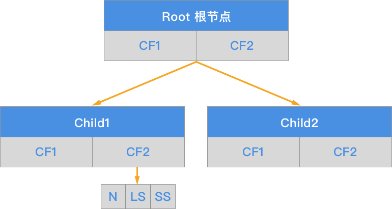
The core of the BIRCH algorithm is to build a CF clustering feature tree based on training samples. The corresponding output of the CF clustering feature tree is a number of CF nodes, and the sample points in each node are a clustering category.

In fact, there is still a lot of content to delve into regarding the characteristics of the CF clustering feature tree and the tree generation process. However, this involves a large amount of mathematical theories and derivation processes, which are not easy to understand, so we will not expand on it here. Students who are interested can read the original paper.

Finally, let’s briefly talk about the advantages of the BIRCH algorithm compared to the Agglomerative algorithm, that is, summarize the necessity of learning the BIRCH algorithm:

1. When building the CF feature tree, the BIRCH algorithm only stores the feature information of the original data and does not need to store the original data information, which is more memory-efficient and computationally efficient.

2. The BIRCH algorithm only needs to traverse the original data once, while the Agglomerative algorithm needs to traverse the data once in each iteration, further highlighting the efficiency of BIRCH.

3. BIRCH belongs to the online learning algorithm and supports the clustering of streaming data. It does not need to know all the data when starting the clustering.

27.18. BIRCH Clustering Implementation

Having said so much above, in summary, BIRCH belongs to a very efficient method among hierarchical clustering algorithms. Next, let’s take a look at how to use the BIRCH class provided by scikit-learn to complete the clustering task.

In this experiment, we will use the handwritten character dataset DIGITS. The full name of this dataset is Pen-Based Recognition of Handwritten Digits Data Set, which is sourced from the UCI open dataset website. The dataset contains digital matrices converted from 1,797 handwritten character images of digits 0 to 9, and the target values are 0 - 9. Since this experiment is to complete a clustering task, actually we want to observe whether there is a spatial connection among characters with the same meaning through their features.

This dataset can be directly called using the load_digits method provided by scikit-learn, which contains three attributes:

Attribute	Description
images	8x8 matrix recording the pixel grayscale values corresponding to each handwritten character image
data	Converting the corresponding 8x8 matrix of images into a row vector
target	Recording the numbers represented by each of the 1,797 images

Next, we visualize the first 5 character images:

digits = datasets.load_digits()

# 查看前 5 个字符
fig, axes = plt.subplots(1, 5, figsize=(12, 4))
for i, image in enumerate(digits.images[:5]):
    axes[i].imshow(image, cmap=plt.cm.gray_r)

As we all know, the data of a handwritten character is represented by an 8x8 matrix.

digits.images[0]

array([[ 0.,  0.,  5., 13.,  9.,  1.,  0.,  0.],
       [ 0.,  0., 13., 15., 10., 15.,  5.,  0.],
       [ 0.,  3., 15.,  2.,  0., 11.,  8.,  0.],
       [ 0.,  4., 12.,  0.,  0.,  8.,  8.,  0.],
       [ 0.,  5.,  8.,  0.,  0.,  9.,  8.,  0.],
       [ 0.,  4., 11.,  0.,  1., 12.,  7.,  0.],
       [ 0.,  2., 14.,  5., 10., 12.,  0.,  0.],
       [ 0.,  0.,  6., 13., 10.,  0.,  0.,  0.]])

If we flatten this matrix, it can be transformed into a 1x64 vector. For such a high-dimensional vector, although the distance can be directly calculated during clustering, it is not possible to well represent the corresponding data points in a two-dimensional plane. Because the points in a two-dimensional plane are only composed of the abscissa and the ordinate.

Therefore, in order to restore the clustering process as much as possible, we need to process the 1x64 row vector (64 dimensions) into a 1x2 row vector (2 dimensions), which is the process of dimensionality reduction.

Since we are reducing the dimensions, then how should we do it? Should we directly take the first two digits, or randomly select two digits? Of course not. Here we learn a new method called PCA (Principal Component Analysis).

27.19. PCA (Principal Component Analysis)

Principal component analysis is a concept in multivariate linear statistics. Its English name is Principal Components Analysis, abbreviated as PCA. Principal component analysis aims to reduce the dimensionality of data and simplify the dataset by retaining the main components in the dataset.

The mathematical principle of principal component analysis is very simple. By performing eigen decomposition on the covariance matrix, the principal components (eigenvectors) and the corresponding weights (eigenvalues) can be obtained. Then, the features corresponding to the smaller eigenvalues (smaller weights) are removed, thus achieving the purpose of reducing the dimensionality of the data.

Principal component analysis usually has two functions:

1. For the purpose of this article, it is convenient to use the data for visualization in a low-dimensional space. Visualization during the clustering process is very necessary.

2. High-dimensional datasets often mean a large consumption of computing resources. By reducing the dimensionality of the data, we can reduce the model learning time without significantly affecting the results.

We will discuss the principle and application of principal component analysis in detail in the subsequent experiments. Therefore, here we directly use the PCA method in scikit-learn to complete:

sklearn.decomposition.PCA(n_components=None, copy=True, whiten=False, svd_solver='auto')

Among them:

• n_components= indicates the number of principal components (features) to be retained.

• copy= indicates whether to perform dimensionality reduction on the original data or a copy of the original data. When the parameter is False, the original data after dimensionality reduction will be changed, and the default here is True.

• whiten= Whitening means reducing the correlation between features and making each feature have the same variance.

• svd_solver= indicates the method for singular value decomposition (SVD). There are 4 parameters, namely: auto, full, arpack, randomized.

When using PCA for dimensionality reduction, we will also use the PCA.fit() method. .fit() is a general method for training models in scikit-learn, but the method itself returns the parameters of the model. Therefore, usually we will use the PCA.fit_transform() method to directly return the data results after dimensionality reduction.

Next, we will perform feature dimensionality reduction on the DIGITS dataset.

from sklearn.decomposition import PCA

# PCA 将数据降为 2 维
pca = PCA(n_components=2)
pca_data = pca.fit_transform(digits.data)
pca_data

array([[ -1.25946669,  21.27488553],
       [  7.95761109, -20.76869371],
       [  6.99192328,  -9.95599129],
       ...,
       [ 10.80128269,  -6.96025666],
       [ -4.87209749,  12.42395892],
       [ -0.34439008,   6.36554125]])

It can be seen that the features of each row have been reduced from the previous 64 to 2. Next, the data after dimensionality reduction will be plotted on a two-dimensional plane.

plt.figure(figsize=(10, 8))
plt.scatter(pca_data[:, 0], pca_data[:, 1])

<matplotlib.collections.PathCollection at 0x15d4070a0>

The above figure shows the data points corresponding to the 1797 samples in the DIGITS dataset after dimensionality reduction by PCA on a two-dimensional plane.

Now, we can directly use BIRCH to cluster the data after dimensionality reduction. Since we know in advance that these are handwritten digit characters, we choose to cluster them into 10 categories. Of course, when clustering, we only know approximately the number of categories to cluster, but we don’t know the corresponding label values of the data.

The main classes and parameters of BIRCH in scikit - learn are as follows:

sklearn.cluster.Birch(threshold=0.5, branching_factor=50, n_clusters=3, compute_labels=True, copy=True)

Among them:

• threshold: The spatial threshold \(\tau\) of each CF. The smaller the parameter value, the larger the scale of the CF feature tree, and the more time and memory will be spent during learning. The default value is 0.5, but if the variance of the samples is large, this default value generally needs to be increased.

• branching_factor: The maximum number of CFs for all nodes in the CF tree. The default value of this parameter is 50. If the sample size is very large, this default value generally needs to be increased.

• n_clusters: Although hierarchical clustering does not require setting the number of categories in advance, the number of categories expected to be queried can be set.

Next, use the BIRCH algorithm to obtain the clustering results of the data after PCA dimensionality reduction:

from sklearn.cluster import Birch

birch = Birch(n_clusters=10)
cluster_pca = birch.fit_predict(pca_data)
cluster_pca

array([3, 0, 0, ..., 0, 5, 9])

Use the obtained clustering results to color the scatter plot.

plt.figure(figsize=(10, 8))
plt.scatter(pca_data[:, 0], pca_data[:, 1], c=cluster_pca)

<matplotlib.collections.PathCollection at 0x15f474910>

# 计算聚类过程中的决策边界
x_min, x_max = pca_data[:, 0].min() - 1, pca_data[:, 0].max() + 1
y_min, y_max = pca_data[:, 1].min() - 1, pca_data[:, 1].max() + 1

xx, yy = np.meshgrid(np.arange(x_min, x_max, 0.4), np.arange(y_min, y_max, 0.4))
temp_cluster = birch.predict(np.c_[xx.ravel(), yy.ravel()])

# 将决策边界绘制出来
temp_cluster = temp_cluster.reshape(xx.shape)
plt.figure(figsize=(10, 8))
plt.contourf(xx, yy, temp_cluster, cmap=plt.cm.bwr, alpha=0.3)
plt.scatter(pca_data[:, 0], pca_data[:, 1], c=cluster_pca, s=15)

# 图像参数设置
plt.xlim(x_min, x_max)
plt.ylim(y_min, y_max)

(-28.494444264008855, 31.092210398474464)

In fact, we can color the scatter plot using the pre-known labels corresponding to each character and compare with the above clustering results.

plt.figure(figsize=(10, 8))
plt.scatter(pca_data[:, 0], pca_data[:, 1], c=digits.target)

<matplotlib.collections.PathCollection at 0x15f4d7ca0>

Comparing the two pictures, you will find that the clustering results of the PCA dimensionality-reduced data generally conform to the distribution trend of the original data. It doesn’t matter that the colors of the color blocks don’t match here, because the order of the original labels and the clustering labels doesn’t match. Just pay attention to the distribution pattern of the data blocks.

However, the scatter plot drawn using the real labels is significantly messier, which is actually caused by PCA dimensionality reduction. Generally, the data we input into the clustering model doesn’t necessarily have to be the dimensionality-reduced data. Now, let’s try reclustering with the original data.

cluster_ori = birch.fit_predict(digits.data)
cluster_ori

array([7, 9, 4, ..., 4, 1, 4])

plt.figure(figsize=(10, 8))
plt.scatter(pca_data[:, 0], pca_data[:, 1], c=cluster_ori)

<matplotlib.collections.PathCollection at 0x15f959ea0>

Now you will find that the clustering results obtained from the experiment are more in line with the distribution pattern of the original dataset. Once again, it should be emphasized that the non-separation of colors here is actually due to the visualization effect on the two-dimensional plane after PCA dimensionality reduction, and it does not represent the real clustering effect.

However, finally, let’s emphasize the usage scenarios of PCA again. Generally, we don’t perform PCA processing as soon as we get the data. We only consider using PCA when the algorithm is not satisfactory, the training time is too long, or visualization is needed, etc. The main reason is that PCA is regarded as a lossy compression of the data, which will cause the loss of the original features of the dataset.

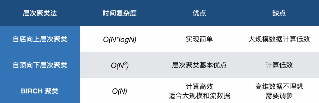
Finally, compare the advantages and disadvantages of the three hierarchical clustering methods in this experiment through a table:

27.20. Summary

In this experiment, we learned about hierarchical clustering methods, especially the agglomerative, divisive, and BIRCH algorithms. Among them, the more commonly used ones are the bottom-up or BIRCH methods, and BIRCH has the characteristic of high computational efficiency. However, BIRCH also has some drawbacks. For example, its clustering effect on high-dimensional data is often not very good, and sometimes we will use Mini Batch K-Means as an alternative.

Related Links

• Hierarchical clustering - Wikipedia

• BIRCH - Wikipedia

---

○ Sharethis article link to your social media, blog, forum, etc. More external links will increase the search engine ranking of this site.

If you find this content helpful, you can buy me a coffee

Previous

26. Image Compression Using K-Means

Next

28. Principal Component Analysis Principle and Applications