Pro Membership

Pro Membership is a membership plan created by the author to maintain and update this tutorial. You can get more benefits and services, click to view details.

25. Implementation and Application of Partitioning Clustering Methods

25.1. Introduction

In the previous courses, we became familiar with the common algorithms in regression and classification. Next, we will lead you to learn and master unsupervised learning: clustering. In this experiment, we will first explain the most commonly used partitioning clustering methods in clustering, and give a detailed introduction to the most representative K-Means algorithm and other members of its family.

25.2. Key Points

• Introduction to Partitioning Clustering

• K-Means Clustering Method

• Visualization of the Process of Moving Centroids

• Implementation of the K-Means++ Algorithm

25.3. Introduction to Partitioning Clustering

Partitioning clustering, as the name implies, divides the dataset into multiple non-overlapping subsets (clusters) through partitioning, with each subset serving as a cluster (category).

During the partitioning process, first the user determines the number \(k\) of subsets to be partitioned, then randomly selects \(k\) points as the centroids of each subset. Next, through an iterative approach: calculate the distances between each point in the dataset and each centroid, and update the positions of the centroids; finally, partition the dataset into \(k\) subsets, that is, partition the data into \(k\) classes.

The criterion for evaluating the quality of the partition is to ensure that the differences between samples within the same partition are as small as possible, and the differences between samples in different partitions are as large as possible.

25.4. K-Means Clustering Method

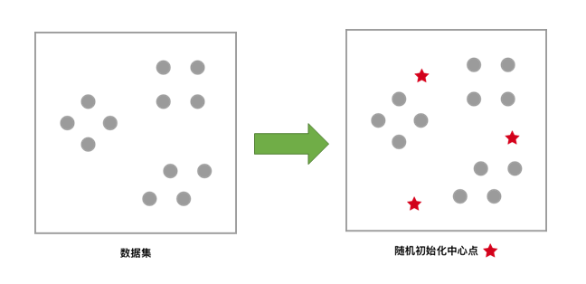
In partitioning clustering, K-Means is the most representative algorithm. The following demonstrates the basic algorithm process of K-Means in the form of pictures. It is hoped that through this simple graphical demonstration, everyone can have a general impression of the principle process of the K-Means method.

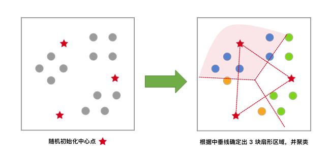
For the unclustered dataset, first randomly initialize K (representing the number of clusters to be formed) centroids, as shown by the red five-pointed stars in the figure.

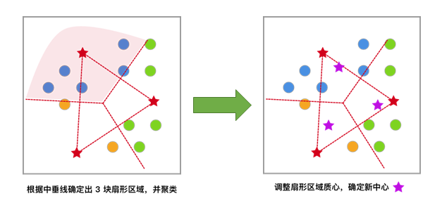
Each sample is clustered according to the centroid closest to itself, which is equivalent to dividing the area by the perpendicular bisector of the line connecting the two centroids.

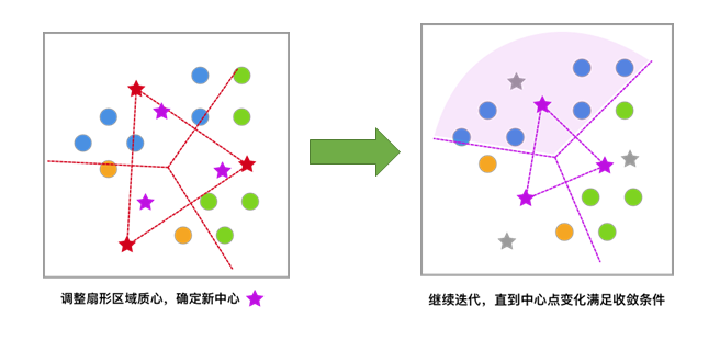
Based on the previous clustering result, move the centroids to the centroid positions of each cluster and use this centroid as the new centroid.

Iterate repeatedly until the change in the centroids meets the convergence condition (the change is very small or almost no change), and finally obtain the clustering result.

After having an intuitive understanding of K-Means, let’s implement it in Python below.

25.5. Generate Sample Data

First, generate the sample data required for this experiment using the make_blobs() function in the scikit-learn module. This method can generate specific clustered data according to our requirements.

data,label = sklearn.datasets.make_blobs(n_samples=100,n_features=2,centers=3,center_box=(-10.0,10.0),random_state=None)   

Among which the parameters are:

• n_samples: Indicates the total number of generated data points, with a default value of 100.

• n_features: Represents the number of features for each sample, with a default value of 2.

• centers: Denotes the number of center points, with a default value of 3.

• center_box: Represents the boundary of each center, with a default range from -10.0 to 10.0.

• random_state: Indicates the random number seed for generating the data.

The return values are:

• data: Represents the data information.

• label: Represents the data category.

According to the above function, generate 200 data points on the interval from 0.0 to 10.0, roughly containing 3 centers. Since it is used to demonstrate the clustering effect, the data labels are not necessary. Assign them to _ when generating the data, and they will not be used later.

from sklearn.datasets import make_blobs

# 构造示例数据
blobs, _ = make_blobs(n_samples=200, centers=3, random_state=18)
blobs[:10]  # 打印出前 10 条数据的信息

array([[ 8.28390539,  4.98011149],
       [ 7.05638504,  7.00948082],
       [ 7.43101466, -6.56941148],
       [ 8.20192526, -6.4442691 ],
       [ 3.15614247,  0.46193832],
       [ 7.7037692 ,  6.14317389],
       [ 5.62705611, -0.35067953],
       [ 7.53828533, -4.86595492],
       [ 8.649291  ,  3.98488194],
       [ 7.91651636,  4.54935348]])

To more intuitively view the data distribution, use Matplotlib to plot the generated data.

import matplotlib.pyplot as plt

%matplotlib inline

plt.scatter(blobs[:, 0], blobs[:, 1], s=20)  # 数据展示

<matplotlib.collections.PathCollection at 0x1573c7a90>

25.6. Randomly Initialize Cluster Centers

When we obtain the data, in accordance with the idea of the partitioning clustering method, we first need to randomly select \(k\) points as the centers of each subset. From the image, it is easy to visually identify that this dataset has 3 subsets. Next, use the NumPy module to randomly generate 3 center points. For easier demonstration, we add a random seed here so that the results are the same every time the code is run.

import numpy as np


def random_k(k, data):
    """
    参数:
    k -- 中心点个数
    data -- 数据集

    返回:
    init_centers -- 初始化中心点
    """
    # 初始化中心点
    prng = np.random.RandomState(27)  # 定义随机种子
    num_feature = np.shape(data)[1]
    # 初始化从标准正态分布返回的一组随机数，为了更加贴近数据集这里乘了一个 5
    init_centers = prng.randn(k, num_feature) * 5
    return init_centers


init_centers = random_k(3, blobs)
init_centers

array([[ 6.42802708, -1.51776689],
       [ 3.09537831,  1.97999275],
       [ 1.11702824, -0.27169709]])

After randomly generating the center points, represent them in the image. Here, red five-pointed stars are also used to represent them.

# 初始中心点展示
plt.scatter(blobs[:, 0], blobs[:, 1], s=20)
plt.scatter(init_centers[:, 0], init_centers[:, 1], s=100, marker="*", c="r")

<matplotlib.collections.PathCollection at 0x1574bfca0>

25.7. Calculate the Distance between Samples and Cluster Centers

To find the most suitable positions of the cluster centers, it is necessary to calculate the distances between each sample and the cluster centers, and then update the positions of the cluster centers based on these distances. Common distance calculation methods include Euclidean distance and cosine similarity. In this experiment, the more common and easier-to-understand Euclidean distance is adopted.

We have learned the specific formula for Euclidean distance before. In fact, it is to square the difference between each corresponding eigenvalue in two data points \(X\) and \(Y\), sum them up, and finally take the square root, which is the Euclidean distance.

def d_euc(x, y):
    """
    参数:
    x -- 数据 a
    y -- 数据 b

    返回:
    d -- 数据 a 和 b 的欧氏距离
    """
    # 计算欧氏距离
    d = np.sqrt(np.sum(np.square(x - y)))
    return d

25.8. Minimize SSE and Update Cluster Centers

Similar to the regression algorithm in Chapter 1 that fits the dataset by minimizing the value of the objective function (e.g., loss function), clustering algorithms usually also optimize an objective function to improve the quality of clustering. In clustering algorithms, the sum of squared errors (SSE) is often used as a criterion to measure the clustering effect. The smaller the SSE, the better the clustering effect. Among them, SSE is expressed as:

\[ SSE(C)=\sum_{k=1}^{K}\sum_{x_{i}\in C_{k}}\left \| x_{i}-c_{k} \right \|^{2} \tag{2} \]

Among them, the dataset \(D = \{ x_{1}, x_{2},..., x_{n} \}\), \(x_{i}\) represents each sample value, \(C\) represents the set of categories generated after K-Means clustering analysis \(C = \{ C_{1}, C_{2},..., C_{K} \}\), and \(c_{k}\) is the center point of category \(C_{k}\). The calculation method of \(c_{k}\) is as follows:

\[ c_{k}=\frac{\sum_{x_{i} \in C_{k}}x_{i}}{I(C_{k})} \tag{3} \]

\(I(C_{k})\) represents the number of data in the \(k\)-th set \(C_{k}\).

Of course, we hope to minimize the SSE function just like minimizing the loss function, so as to find the optimal clustering model. However, it is not easy to find its minimum value, which is an NP-hard (Non-deterministic Polynomial) problem. The NP-hard problem is a classic graph theory problem, and so far, no perfect and effective algorithm has been found.

Next, we implement the update of the center point in code:

def update_center(clusters, data, centers):
    """
    参数:
    clusters -- 每一点分好的类别
    data -- 数据集
    centers -- 中心点集合

    返回:
    new_centers -- 新中心点集合
    """
    # 中心点的更新
    num_centers = np.shape(centers)[0]  # 中心点的个数
    num_features = np.shape(centers)[1]  # 每一个中心点的特征数
    container = []

    for x in range(num_centers):
        each_container = []
        container.append(each_container)  # 首先创建一个容器，将相同类别数据存放到一起

    for i, cluster in enumerate(clusters):
        container[cluster].append(data[i])

    new_centers = []
    for i in range(len(container)):
        each_center = np.mean(container[i], axis=0)  # 计算每一子集中数据均值作为中心点
        new_centers.append(each_center)

    return np.vstack(new_centers)  # 使用 np.vstack 将数组垂直堆叠

25.9. K-Means Clustering Algorithm Implementation

The K-Means algorithm uses an iterative algorithm, avoiding optimizing the SSE function. By continuously moving the distance of the center point, the clustering effect is finally achieved. First, let’s take a look at the algorithm process:

1. Initialize the center points: Determine that the dataset may be divided into \(k\) subsets, and randomly generate \(k\) random points as the center points for each subset.

2. Calculate distances and assign class labels: Calculate the distances between the samples and each center point, and assign the class represented by the nearest center point as the class label of the sample.

3. Update the positions of the center points: Calculate the mean of all samples in each class as the new position of the center point.

4. Repeat steps 2 and 3 until the positions of the center points no longer change.

Next, implement the algorithm according to the process.

def kmeans_cluster(data, init_centers, k):
    """
    参数:
    data -- 数据集
    init_centers -- 初始化中心点集合
    k -- 中心点个数

    返回:
    centers_container -- 每一次更新中心点的集合
    cluster_container -- 每一次更新类别的集合
    """
    # K-Means 聚类
    max_step = 50  # 定义最大迭代次数，中心点最多移动的次数。
    epsilon = 0.001  # 定义一个足够小的数，通过中心点变化的距离是否小于该数，判断中心点是否变化。

    old_centers = init_centers

    centers_container = []  # 建立一个中心点容器，存放每一次变化后的中心点，以便后面的绘图。
    cluster_container = []  # 建立一个分类容器，存放每一次中心点变化后数据的类别
    centers_container.append(old_centers)

    for step in range(max_step):
        cluster = np.array([], dtype=int)
        for each_data in data:
            distances = np.array([])
            for each_center in old_centers:
                temp_distance = d_euc(each_data, each_center)  # 计算样本和中心点的欧式距离
                distances = np.append(distances, temp_distance)
            lab = np.argmin(distances)  # 返回距离最近中心点的索引，即按照最近中心点分类
            cluster = np.append(cluster, lab)
        cluster_container.append(cluster)

        new_centers = update_center(cluster, data, old_centers)  # 根据子集分类更新中心点

        # 计算每个中心点更新前后之间的欧式距离
        difference = []
        for each_old_center, each_new_center in zip(old_centers, new_centers):
            difference.append(d_euc(each_old_center, each_new_center))

        if (np.array(difference) < epsilon).all():  # 判断每个中心点移动是否均小于 epsilon
            return centers_container, cluster_container

        centers_container.append(new_centers)
        old_centers = new_centers

    return centers_container, cluster_container

After completing the K-Means clustering function, next use the function to obtain the positions of the final center points.

# 计算最终中心点
centers_container, cluster_container = kmeans_cluster(blobs, init_centers, 3)
final_center = centers_container[-1]
final_cluster = cluster_container[-1]
final_center

array([[ 7.67007252, -6.44697348],
       [ 6.83832746,  4.98604668],
       [ 3.28477676,  0.15456871]])

Finally, we draw the centers obtained from clustering onto the original image to see the clustering effect.

# 可视化展示
plt.scatter(blobs[:, 0], blobs[:, 1], s=20, c=final_cluster)
plt.scatter(final_center[:, 0], final_center[:, 1], s=100, marker="*", c="r")

<matplotlib.collections.PathCollection at 0x15755ed40>

So far, the process of K-Means clustering has been completed. To help everyone understand, we try to draw the process of the movement and change of the center points during the K-Means clustering process.

num_axes = len(centers_container)

fig, axes = plt.subplots(1, num_axes, figsize=(20, 4))

axes[0].scatter(blobs[:, 0], blobs[:, 1], s=20, c=cluster_container[0])
axes[0].scatter(init_centers[:, 0], init_centers[:, 1], s=100, marker="*", c="r")
axes[0].set_title("initial center")

for i in range(1, num_axes - 1):
    axes[i].scatter(blobs[:, 0], blobs[:, 1], s=20, c=cluster_container[i])
    axes[i].scatter(
        centers_container[i][:, 0], centers_container[i][:, 1], s=100, marker="*", c="r"
    )
    axes[i].set_title("step {}".format(i))

axes[-1].scatter(blobs[:, 0], blobs[:, 1], s=20, c=cluster_container[-1])
axes[-1].scatter(final_center[:, 0], final_center[:, 1], s=100, marker="*", c="r")
axes[-1].set_title("final center")

Text(0.5, 1.0, 'final center')

You will be surprised to find that for the example dataset, although the maximum number of iterations max_step was previously set to 50, in fact, the K-Means algorithm converges after only 3 iterations. There are mainly two reasons:

• The initial positions of the center points are well-chosen and evenly distributed within the data range. If the initial center points are concentrated in a certain corner, the number of iterations will definitely increase.

• The distribution of the example data is regular and simple, enabling convergence without the need for many iterations.

25.10. Selection of the K Value in K-Means Algorithm Clustering

I wonder if you still remember that when we learned about the K-Nearest Neighbors classification algorithm before, we talked about the selection of the K value. When using the K-Means algorithm for clustering, since we need to determine the number of randomly initialized center points in advance, we also face the problem of K value selection.

When looking for the K value before, we thought it should be clustered into 3 categories by visual inspection. So, what if we set the number of clusters to 5? This time, we try to complete the clustering using the K-Means algorithm in the scikit-learn module.

sklearn.cluster.k_means(X, n_clusters)

Among them, the parameters are:

• X: Represents the data to be clustered.

• n_clusters: Represents the number of clusters, that is, the K value.

The return value contains:

• centroid: Represents the coordinates of the center point.

• label: Represents the category of each sample after clustering.

• inertia: The sum of the squares of the distances from each sample to the nearest center point, i.e., SSE.

# 用 scikit-learn 聚类并绘图
from sklearn.cluster import k_means

model = k_means(blobs, n_clusters=5, n_init="auto")

centers = model[0]
clusters_info = model[1]
plt.scatter(blobs[:, 0], blobs[:, 1], s=20, c=clusters_info)
plt.scatter(centers[:, 0], centers[:, 1], s=100, marker="*", c="r")

<matplotlib.collections.PathCollection at 0x15a853c40>

Judging from the picture, the effect of clustering into 5 categories is significantly worse than that of clustering into 3 categories. Of course, we can roughly tell with the naked eye in advance that the data is approximately in 3 clusters.

In the actual application process, if it is impossible to judge by the naked eye how many categories the data should be clustered into? Or high-dimensional data cannot be visually displayed. Facing such a situation, we have to judge the size of the K value from the perspective of numerical calculation. Next, the experiment will introduce the “elbow method”, which can help us select the K value.

When using the K-Means algorithm for clustering, we can calculate the sum of squared errors (SSE), which is the sum of the squares of the distances from each sample to the nearest centroid, after clustering with different values of K.

As the value of K increases, that is, as the number of categories increases, the within-class similarity within each category also increases, and the resulting change in SSE decreases monotonically. You can imagine that when the number of clustering categories is the same as the total number of samples, that is, when one sample represents one category, this value will become 0.

Next, we will plot the distances between samples and their nearest centroids under different numbers of clusters through code.

index = []  # 横坐标数组
inertia = []  # 纵坐标数组

# K 从 1~ 6 聚类
for i in range(6):
    model = k_means(blobs, n_clusters=i + 1, n_init="auto")
    index.append(i + 1)
    inertia.append(model[2])

# 绘制折线图
plt.plot(index, inertia, "-o")

[<matplotlib.lines.Line2D at 0x15a8ea410>]

As can be seen from the above figure, as expected, the total distance between samples and their nearest centroids decreases as the value of K increases. Now, recall the criteria for evaluating the quality of a partition in the clustering division of this experiment: “Ensure that the differences between samples in the same partition are as small as possible, and the differences between samples in different partitions are as large as possible.”

When the value of K is larger, it better satisfies the condition that “the differences between samples in the same partition are as small as possible”. When the value of K is smaller, it better satisfies the condition that “the differences between samples in different partitions are as large as possible (the maximum distortion degree)”. So, how can we achieve a balance between the two extremes?

Therefore, in the graph plotted by SSE, we call the point with the maximum distortion degree the “elbow”. As can be seen from the graph, the “elbow” here is at K = 3 (the smallest interior angle and the largest curvature). This also indicates that clustering the samples into 3 categories is the best choice (K = 2 is relatively close). This is the so-called “elbow method”. Do you understand?

25.11. K-Means++ Clustering Algorithm

As the amount of data grows and the number of classification categories increases, since the initial centroids in K-Means are randomly selected, there often arise problems such as: multiple centroids in a relatively large subset, while a single centroid is shared by multiple other smaller subsets. That is, the problem that the algorithm gets stuck in a local optimal solution rather than reaching the global optimal solution.

The main reason for this problem is that: some centroids are too close to each other during initialization. Let’s further understand this through an example below.

Similarly, we first use the make_blobs function in the scikit-learn module to generate the data required for this experiment. This time, 800 data points are generated, divided into 5 clusters.

blobs_plus, _ = make_blobs(n_samples=800, centers=5, random_state=18)  # 生成数据
plt.scatter(blobs_plus[:, 0], blobs_plus[:, 1], s=20)  # 将数据可视化展示

<matplotlib.collections.PathCollection at 0x15a962530>

25.12. Random Initialization of Centroids

It can be easily observed from the data point distribution that the number of clusters should be 5. We first use the method of randomly initializing centroids in K-Means to complete the clustering:

km_init_center = random_k(5, blobs_plus)

plt.scatter(blobs_plus[:, 0], blobs_plus[:, 1], s=20)
plt.scatter(km_init_center[:, 0], km_init_center[:, 1], s=100, marker="*", c="r")

<matplotlib.collections.PathCollection at 0x15a9f4eb0>

25.13. K-Means Clustering

Use the traditional K-Means algorithm to cluster the dataset with the number of clusters being 5.

km_centers, km_clusters = kmeans_cluster(blobs_plus, km_init_center, 5)
km_final_center = km_centers[-1]
km_final_cluster = km_clusters[-1]
plt.scatter(blobs_plus[:, 0], blobs_plus[:, 1], s=20, c=km_final_cluster)
plt.scatter(km_final_center[:, 0], km_final_center[:, 1], s=100, marker="*", c="r")

<matplotlib.collections.PathCollection at 0x15aa72ec0>

After clustering with the traditional K-Means algorithm, you will find that the clustering result is different from what we expected. The result we expected should be like this:

plt.scatter(blobs_plus[:, 0], blobs_plus[:, 1], s=20, c=_)

<matplotlib.collections.PathCollection at 0x15aaf4be0>

By comparing the two graphs of K-Means clustering and the expected clustering, it can be intuitively seen that the K-Means algorithm obviously fails to achieve the optimal clustering effect, and the problem of local optimal solution mentioned at the beginning of this chapter occurs.

The local optimum problem can be solved by SSE, that is, running the K-Means algorithm for clustering multiple times on the same dataset, and then selecting the run with the smallest SSE as the final clustering result. Although it is very difficult to find the optimal solution through SSE, it is very easy to judge the optimal solution through SSE.

However, when dealing with larger datasets where each run of the K-Means algorithm takes a significant amount of time, using multiple runs to determine the optimal solution through SSE is obviously not a good choice. Is there a method that can effectively avoid the occurrence of the local optimum problem when initializing the center points?

Based on K-Means, D. Arthur et al. proposed the K-Means++ algorithm in 2007. The K-Means++ algorithm mainly improves the problem of initializing the center points, thus solving the problem of local optimal solutions at the source.

25.14. K-Means++ Algorithm Process

K-Means++ has made improvements in initializing the center points compared to K-Means, and is the same as K-Means in other aspects.

1. Randomly select a sample point in the dataset as the first initialized cluster center.

2. Calculate the distance \(D(x)\) between the non-center points in the sample and the nearest center point and save it in an array. Add up these distances in the array to get \(sum(D(x))\).

3. Take a random value \(R\) within the range of \(sum(D(x))\), and repeatedly calculate \(R = R - D(x)\) until \(R \leq 0\). Select the point at this time as the next center point.

4. Repeat steps 2 and 3 until \(K\) cluster centers are determined.

5. For the \(K\) initialized cluster centers, use the K-Means algorithm to calculate the final cluster centers.

After looking at the entire algorithm process, a question may arise: To avoid the initial points being too close, wouldn’t it be better to directly select the points that are the farthest apart? Why introduce a random value \(R\)?

In fact, when using the method of directly selecting the points that are the farthest apart as the initial points, it is vulnerable to the interference of outliers in the dataset. The method of introducing a random value \(R\) is used to avoid the interference of the outliers contained in the dataset on the goal of selecting the center points that are the farthest apart in the algorithm idea.

Compared with normal data points, the calculated distance \(D(x)\) of outliers is relatively large. In the selection process, the probability of it being selected is relatively high. However, outliers only account for a small part of the entire dataset, and most are still normal points. Thus, the high probability caused by the large distance of outliers is balanced by the large number of normal points, ensuring the balance of the entire algorithm.

25.15. K-Means++ Algorithm Implementation

After initializing the sample points in K-Means++, calculate the sum of the distances between other samples and their nearest center points for the selection of the next center point. The following is the implementation in Python:

def get_sum_dis(centers, data):
    """
    参数:
    centers -- 中心点集合
    data -- 数据集

    返回:
    np.sum(dis_container) -- 样本距离最近中心点的距离之和
    dis_container -- 样本距离最近中心点的距离集合
    """

    dis_container = np.array([])
    for each_data in data:
        distances = np.array([])
        for each_center in centers:
            temp_distance = d_euc(each_data, each_center)  # 计算样本和中心点的欧式距离
            distances = np.append(distances, temp_distance)
        lab = np.min(distances)
        dis_container = np.append(dis_container, lab)
    return np.sum(dis_container), dis_container

Next, we initialize the center points:

def get_init_center(data, k):
    """
    参数:
    data -- 数据集
    k -- 中心点个数

    返回:
    np.array(center_container) -- 初始化中心点集合
    """
    # K-Means++ 初始化中心点
    seed = np.random.RandomState(20)
    p = seed.randint(0, len(data))
    first_center = data[p]

    center_container = []
    center_container.append(first_center)

    for i in range(k - 1):
        sum_dis, dis_con = get_sum_dis(center_container, data)
        r = np.random.randint(0, sum_dis)
        for j in range(len(dis_con)):
            r = r - dis_con[j]
            if r <= 0:
                center_container.append(data[j])
                break
            else:
                pass

    return np.array(center_container)

After implementing the K-Means++ center point initialization function, obtain the initialized center point coordinates based on the generated data.

plus_init_center = get_init_center(blobs_plus, 5)
plus_init_center

array([[ 4.1661903 ,  0.81807492],
       [-5.66400236, -8.74915813],
       [ 2.97927567,  9.7835682 ],
       [ 6.31810657,  5.42968049],
       [ 8.39657941, -8.03027348]])

To let you see the process of initializing the center points in K-Means++ more clearly, we use Matplotlib to display it.

num = len(plus_init_center)

fig, axes = plt.subplots(1, num, figsize=(25, 4))

axes[0].scatter(blobs_plus[:, 0], blobs_plus[:, 1], s=20, c="b")
axes[0].scatter(
    plus_init_center[0, 0], plus_init_center[0, 1], s=100, marker="*", c="r"
)
axes[0].set_title("first center")

for i in range(1, num):
    axes[i].scatter(blobs_plus[:, 0], blobs_plus[:, 1], s=20, c="b")
    axes[i].scatter(
        plus_init_center[: i + 1, 0],
        plus_init_center[: i + 1, 1],
        s=100,
        marker="*",
        c="r",
    )
    axes[i].set_title("step{}".format(i))

axes[-1].scatter(blobs_plus[:, 0], blobs_plus[:, 1], s=20, c="b")
axes[-1].scatter(
    plus_init_center[:, 0], plus_init_center[:, 1], s=100, marker="*", c="r"
)
axes[-1].set_title("final center")

Text(0.5, 1.0, 'final center')

From the above figure, we can see the changes in the points. That is, except for the initially randomly selected points, each subsequent point is selected as far away as possible. This can well ensure the dispersion of the initial center points.

By executing the code multiple times, it can be seen that when using K-Means++, it is also possible for two center points to be relatively close. Therefore, in extreme cases, the problem of local optimality may also occur. However, compared with the random selection of the K-Means algorithm, the initialization of the center points in K-Means++ will greatly reduce the probability of the occurrence of the local optimality problem.

After initializing the center points through the K-Means++ algorithm, next we perform clustering on the data using the K-Means algorithm.

plus_centers, plus_clusters = kmeans_cluster(blobs_plus, plus_init_center, 5)
plus_final_center = plus_centers[-1]
plus_final_cluster = plus_clusters[-1]

plt.scatter(blobs_plus[:, 0], blobs_plus[:, 1], s=20, c=plus_final_cluster)
plt.scatter(plus_final_center[:, 0], plus_final_center[:, 1], s=100, marker="*", c="r")

<matplotlib.collections.PathCollection at 0x15af453f0>

In the K-Means++ algorithm, we still can’t completely avoid the instability caused by randomly selecting the center points, so occasionally we will also get less satisfactory results. Of course, the probability of the K-Means++ algorithm getting less satisfactory clustering is much lower than that of the K-Means algorithm. Therefore, if you don’t get a good clustering effect, you can try initializing the center points again.

25.16. Mini-Batch K-Means Clustering Algorithm

In the era when “big data” is so popular, can the K-Means algorithm still handle big data as excellently as before? Now let’s review the algorithm principle of K-Means again: First, calculate the distance between each sample and all the center points, find the nearest center point by comparison, store and classify the distance to the nearest center point. Then, update the position of the center point through the feature values of the samples in the same category. Thus, one iteration is completed, and after multiple iterations, clustering is finally performed.

From the above description, do you feel how much computational effort is involved in the process of continuously calculating distances? Well, imagine when the data volume reaches hundreds of thousands, millions, or tens of millions, and if each piece of data has hundreds of features, this will consume a huge amount of computing resources.

To solve the clustering problem of large-scale data, we can use another variant of K-Means, Mini Batch K-Means, to complete it.

Its algorithm principle is also very simple: In each iteration process, a small batch of data is randomly sampled from the dataset to form a mini-batch dataset, and this part of the dataset is used for distance calculation and center point update. Since it is randomly sampled each time, the data sampled each time can well represent the characteristics of the original dataset.

Next, we generate a set of test data and test the differences in clustering time and SSE between the K-Means algorithm and Mini Batch K-Means on the same set of data. Since the parameters of the MiniBatchKMeans() and KMeans() methods in scikit-learn are almost the same, they will not be elaborated here.

import time
from sklearn.cluster import MiniBatchKMeans, KMeans


test_data, _ = make_blobs(
    20000, n_features=2, cluster_std=0.9, centers=5, random_state=20
)

km = KMeans(n_clusters=5, n_init="auto")
mini_km = MiniBatchKMeans(n_clusters=5, n_init="auto")

fig, axes = plt.subplots(nrows=1, ncols=2, figsize=(10, 5))

for i, model in enumerate([km, mini_km]):
    t0 = time.time()
    model.fit(test_data)
    t1 = time.time()
    t = t1 - t0
    sse = model.inertia_
    axes[i].scatter(test_data[:, 0], test_data[:, 1], c=model.labels_)
    axes[i].set_xlabel("time: {:.4f} s".format(t))
    axes[i].set_ylabel("SSE: {:.4f}".format(sse))

axes[0].set_title("K-Means")
axes[1].set_title("Mini Batch K-Means")

Text(0.5, 1.0, 'Mini Batch K-Means')

The above is the clustering of 2,000 pieces of data using K-Means and Mini Batch K-Means respectively. It can be seen from the image that Mini Batch K-Means is significantly faster than K-Means in terms of training time (more than twice as fast), and the SSE values obtained by clustering are relatively close.

25.17. Summary

In this section of the experiment, we learned the principle of the K-Means algorithm in the partitioning clustering algorithm and implemented it in the Python language. Subsequently, based on the deficiencies of the K-Means algorithm, we learned its variants K-Means++ and Mini Batch K-Means in its family. Although the algorithm principle is easy to understand, more practical exercises are needed to truly master it.

Related Links

• K-Means Algorithm - Wikipedia

• The 5 Clustering Algorithms Data Scientists Need to Know

• Visualizing K-Means Clustering

---

○ Sharethis article link to your social media, blog, forum, etc. More external links will increase the search engine ranking of this site.

If you find this content helpful, you can buy me a coffee

Previous

24. Quickly Select Models Using Cross-Validation

Next

26. Image Compression Using K-Means