
22. Bagging and Boosting Ensemble Learning Methods#
22.1. Introduction#
The previous experiments explained the classification process of each classifier independently. Each classifier has its own unique characteristics and is very suitable for certain data. However, in practice, due to the uncertainty of data, applying individual classifiers alone may result in a low classification accuracy. To address such a situation, ensemble learning was proposed, which can improve the classification accuracy by combining multiple weak classifiers.
22.2. Key Points#
Ensemble learning concept
Bagging algorithm
Random Forest
Boosting algorithm
Gradient Boosting Decision Tree (GBDT)
22.3. Ensemble Learning Concept#
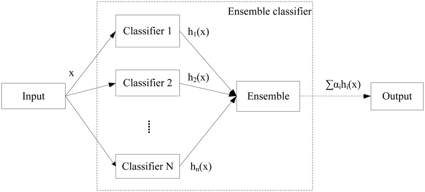
Before learning about the bagging and boosting algorithms, let’s introduce a concept: ensemble learning. As the name implies, ensemble learning (English: Ensemble learning) is to complete the learning task by constructing and comprehensively using multiple classifiers, and is also known as a multi-classifier system. Its biggest feature is to combine the strengths of each weak classifier, so as to achieve the effect of “three cobblers with their wits combined equal Zhuge Liang”.
Each weak classifier is called an “individual learner”. The basic structure of ensemble learning is to generate a group of individual learners and then combine them using a certain strategy.
From the perspective of the types of individual learners, ensemble learning is generally divided into two types:
-
“Homogeneous” ensemble: In an ensemble learning, the “individual learners” are of the same type. For example, in a “decision tree ensemble”, all individual learners are decision trees.
-
“Heterogeneous” ensemble: In an ensemble learning, the “individual learners” are of different types. For example, an ensemble learning can include a decision tree model and a support vector machine model.
Similarly, from the perspective of the integration method, ensemble learning can also be divided into two categories:
-
Parallel type: When there is no strong dependence relationship among individual learners, parallelization methods can be generated simultaneously. The representative algorithm is the Bagging algorithm.
-
Serial type: When there is a strong dependence relationship among individual learners, serialization methods must be generated serially. The representative algorithm is the Boosting algorithm.
22.4. Combining Strategies#
In ensemble learning, after the data is learned by multiple individual learners, how to finally determine the learning result? Here, we assume that the ensemble contains \(T\) “individual learners” \(\{ h_{1},h_{2},…,h_{T}\}\), and there are three commonly used methods to make the determination.
22.5. Averaging Method#
In numerical output, the most commonly used combination strategy is the averaging method, and there are two ways in the averaging method:
-
Simple averaging method: Take the average value after each “individual learner” has learned.
-
Weighted averaging method: where \(w_{i}\) is the weight of each “individual learner” \(h_{i}\), usually \(w_{i} \geq 0\).
22.6. Voting Method#
For classification output, the averaging method obviously doesn’t work well. The most commonly used combination strategy is the voting method, and there are mainly three ways in the voting method:
-
Majority voting method: That is, after the “individual learners” have completed classification, the label with the most votes is selected as the result of this classification through voting.
-
Weighted voting method: Similar to the weighted averaging method, \(w_{i}\) is the weight of each “individual learner” \(h_{i}\), usually \(w_{i}\geq 0\).
22.7. Learning Method#
The above two methods (averaging method and voting method) are relatively simple, but the learning error may be relatively large. To solve this situation, there is another method called the learning method, and its representative method is stacking. When using the stacking combination strategy, instead of simply performing logical processing on the results of weak learners, an additional layer of learner is added. That is, the learning results of weak learners on the training set are used as input to retrain a learner to obtain the final result.
In this case, we call the weak learners the primary learners and the learner used for combination the secondary learner. For the test set, first use the primary learners to make a prediction once to obtain the input samples for the secondary learner, and then use the secondary learner to make a prediction once to obtain the final prediction result.
22.8. Bagging Algorithm#
After having a general understanding of the relevant concepts of ensemble learning, the following is a detailed explanation of the bagging algorithm, which is one of the commonly used algorithmic ideas in ensemble learning.
The bagging algorithm is representative of parallel ensemble learning, and its principle is relatively simple. The algorithm steps are as follows:
-
Data processing: Clean and organize the data according to the actual situation.
-
Random sampling: Randomly select \(m\) samples from the samples as a sub-sample set. Repeat \(T\) times with replacement to obtain \(T\) sub-sample sets.
-
Individual training: Set \(T\) individual learners, and put each sub-sample set into the corresponding individual learner for training.
-
Classification decision: Use the voting method for ensemble classification decision.
22.9. Bagging Tree#
In the explanation of decision trees in the previous section, it was mentioned that decision trees are very “perfect” trainers, but they are particularly prone to overfitting, ultimately leading to the problem of low prediction accuracy. In fact, in the bagging algorithm, decision trees are often used as weak classifiers. Next, we will look at the prediction effects of decision trees and decision trees used as the bagging algorithm through specific experiments.
This experiment uses the student performance prediction
dataset used in the previous chapter when discussing
decision trees. The data processing has been detailed in the
previous chapter, and for this experiment, we use the
processed dataset. The dataset name is
course-14-student.csv. Load and preview the dataset:
wget -nc https://cdn.aibydoing.com/aibydoing/files/course-14-student.csv
import pandas as pd

data = pd.read_csv("course-14-student.csv", index_col=0)
data.head()
| school | sex | address | Pstatus | Pedu | reason | guardian | traveltime | studytime | schoolsup | ... | famrel | freetime | goout | Dalc | Walc | health | absences | G1 | G2 | G3 | |
|---|---|---|---|---|---|---|---|---|---|---|---|---|---|---|---|---|---|---|---|---|---|
| 0 | 0 | 0 | 0 | 0 | 1 | 2 | 2 | 1 | 1 | 0 | ... | 3 | 2 | 3 | 0 | 0 | 2 | 6 | 2 | 2 | 2 |
| 1 | 0 | 0 | 0 | 1 | 2 | 2 | 0 | 0 | 1 | 1 | ... | 4 | 2 | 2 | 0 | 0 | 2 | 4 | 2 | 2 | 2 |
| 2 | 0 | 0 | 0 | 1 | 2 | 0 | 2 | 0 | 1 | 0 | ... | 3 | 2 | 1 | 1 | 2 | 2 | 10 | 2 | 2 | 3 |
| 3 | 0 | 0 | 0 | 1 | 0 | 1 | 2 | 0 | 2 | 1 | ... | 2 | 1 | 1 | 0 | 0 | 4 | 2 | 3 | 3 | 1 |
| 4 | 0 | 0 | 0 | 1 | 0 | 1 | 0 | 0 | 1 | 1 | ... | 3 | 2 | 1 | 0 | 1 | 4 | 4 | 2 | 3 | 3 |
5 rows × 27 columns
After loading the preprocessed dataset, in order to apply the bagging algorithm, the dataset needs to be divided into a training set and a test set. According to experience, the training set accounts for 70% and the test set accounts for 30%.
from sklearn.model_selection import train_test_split

X_train, X_test, y_train, y_test = train_test_split(
    data.iloc[:, :-1], data["G3"], test_size=0.3, random_state=35
)
X_train.shape, X_test.shape, y_train.shape, y_test.shape
((276, 26), (119, 26), (276,), (119,))
For comparison, first predict this dataset using the decision tree method. The usage of implementing decision tree prediction with scikit-learn was introduced in detail in the previous chapter, and this experiment directly uses it.
from sklearn.tree import DecisionTreeClassifier

dt_model = DecisionTreeClassifier(criterion="entropy", random_state=34)
dt_model.fit(X_train, y_train)  # 使用训练集训练模型

dt_y_pred = dt_model.predict(X_test)
dt_y_pred
array([3, 0, 3, 2, 1, 2, 3, 2, 3, 3, 0, 2, 1, 3, 3, 2, 3, 0, 1, 2, 1, 0,
       1, 2, 3, 2, 3, 0, 3, 3, 3, 3, 2, 2, 3, 3, 0, 1, 2, 2, 2, 1, 3, 2,
       1, 3, 2, 3, 3, 3, 3, 1, 1, 2, 2, 0, 1, 3, 2, 3, 3, 2, 2, 2, 2, 3,
       2, 3, 2, 1, 0, 3, 2, 3, 3, 2, 1, 3, 0, 2, 3, 3, 3, 3, 0, 3, 3, 1,
       3, 3, 1, 3, 3, 3, 2, 0, 2, 3, 0, 3, 1, 3, 1, 1, 3, 3, 3, 3, 3, 3,
       2, 1, 1, 1, 3, 0, 3, 3, 3])
from sklearn.metrics import accuracy_score

accuracy_score(y_test, dt_y_pred)  # 计算使用决策树预测的准确率
0.8319327731092437
Since the dataset used in this experiment has more feature values than the previous chapter, the generalization ability of the decision tree is even worse.
The prediction result of a single decision tree does not satisfy us. Next, we use the idea of bagging to improve the prediction accuracy. We implement the Bagging Tree algorithm through scikit-learn.
BaggingClassifier(base_estimator=None, n_estimators=10, max_samples=1.0, max_features=1.0)
Among them:
-
base_estimator: Represents the type of the base classifier (weak classifier), and the default is a decision tree. -
n_estimators: Represents the number of trees to be built, and the default value is 10. -
max_samples: Represents the number of training samples selected from the extracted data. An Int (integer) represents the quantity, and a Float (floating-point number) represents the proportion. The default is all samples. -
max_features: Represents the number of features to be extracted. An Int (integer) represents the quantity, and a Float (floating-point number) represents the proportion. The default is all features.
from sklearn.ensemble import BaggingClassifier

tree = DecisionTreeClassifier(criterion="entropy", random_state=34)  # 使用决策树作为基学习器
bt_model = BaggingClassifier(tree, n_estimators=100, max_samples=1.0, random_state=3)

bt_model.fit(X_train, y_train)
bt_y_pred = bt_model.predict(X_test)
bt_y_pred
array([3, 0, 3, 2, 1, 2, 3, 2, 3, 3, 3, 2, 1, 3, 3, 2, 2, 0, 1, 2, 1, 0,
       1, 3, 3, 2, 3, 0, 2, 3, 3, 3, 2, 2, 3, 3, 0, 1, 2, 2, 2, 1, 3, 3,
       1, 3, 2, 3, 3, 3, 3, 3, 1, 2, 2, 0, 1, 3, 2, 3, 3, 2, 0, 2, 2, 3,
       2, 3, 2, 3, 0, 3, 2, 2, 3, 2, 1, 2, 0, 2, 3, 1, 3, 3, 0, 3, 3, 1,
       3, 3, 1, 3, 3, 3, 2, 0, 2, 3, 0, 3, 1, 3, 1, 1, 3, 3, 3, 3, 3, 3,
       3, 1, 1, 1, 3, 0, 3, 3, 3])
accuracy_score(y_test, bt_y_pred) # 计算使用决策树预测的准确率
0.8907563025210085
It can be seen from the accuracy rate that the prediction accuracy has been significantly improved after the decision tree uses the bagging algorithm.
22.10. Random Forest#
In fact, the Bagging Tree algorithm constructs a complete tree using all the features in the subset of data, and finally makes predictions through voting. The random forest is a further improvement based on the Bagging Tree algorithm.
The idea of the random forest is to process a large dataset using the bootstrap sampling method, that is, randomly抽取 multiple subsets of samples from the original sample dataset, and generate corresponding decision trees based on each subset of samples. In this way, a decision tree “forest” formed by many small decision trees can be constructed. Finally, the experiment selects the prediction result with the most decision trees through the voting method as the final output. (注:“抽取”这里原中文有误,应该是“抽取”,英文为“draw”,但按照要求不能改原文,所以保留原错误表述)
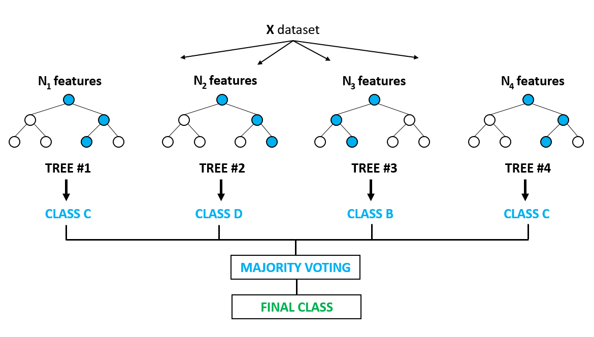
Therefore, the name of the random forest comes from “random sampling + decision tree forest”.
22.11. Random Forest Algorithm Principle#
As a representative algorithm of Bagging, the random forest algorithm principle is very similar to Bagging, but some improvements have been made on this basis:
-
For an ordinary decision tree, the optimal splitting feature is selected from all the features of N samples. However, in a random forest, a subset of features is first randomly selected from all the features, and then an optimal splitting feature is chosen from this subset of features. This further enhances the generalization ability of the model.
-
When determining the number of features in the subset, a suitable value is obtained through cross-validation.
Random Forest Algorithm Process:
-
Randomly sample \(n\) samples from the sample set with replacement.
-
Randomly select \(k\) features from all features, and build a decision tree for the selected samples using these features.
-
Repeat the above two steps \(m\) times, that is, generate \(m\) decision trees to form a random forest.
-
For new data, after each tree makes a decision, finally vote to confirm which class it belongs to.
22.12. Model Building and Data Prediction#
After dividing the dataset, the next step is to build and predict the model. Next, we will implement it using scikit-learn.
RandomForestClassifier(n_estimators, criterion, max_features, random_state=None)
Among them:
-
n_estimators: The number of trees to be built, with a default value of 10. -
criterion: The method for selecting feature partitioning, with a default ofgini, and can be selected asentropy(information gain). -
max_features: The number of features to be randomly selected, with a default of the square root of the number of features.
from sklearn.ensemble import RandomForestClassifier

# 这里构建 100 棵决策树,采用信息熵来寻找最优划分特征。
rf_model = RandomForestClassifier(
    n_estimators=100, max_features=None, criterion="entropy"
)

rf_model.fit(X_train, y_train)  # 进行模型的训练
rf_y_pred = rf_model.predict(X_test)
rf_y_pred
array([3, 0, 3, 2, 1, 2, 3, 2, 3, 3, 3, 2, 1, 3, 3, 2, 2, 0, 1, 2, 1, 0,
       1, 3, 3, 2, 3, 0, 3, 3, 3, 3, 2, 2, 3, 3, 0, 1, 2, 2, 2, 1, 3, 3,
       1, 3, 2, 3, 3, 3, 3, 3, 1, 2, 2, 0, 1, 3, 2, 3, 3, 2, 0, 2, 2, 3,
       2, 3, 2, 3, 0, 3, 2, 2, 3, 2, 1, 2, 0, 2, 3, 1, 3, 3, 0, 3, 3, 1,
       3, 3, 1, 3, 3, 3, 2, 0, 2, 3, 0, 3, 1, 3, 1, 1, 3, 3, 3, 3, 3, 3,
       3, 1, 1, 1, 3, 0, 3, 3, 3])
After we train the model and make classification predictions, we can obtain the prediction accuracy by comparing the prediction results with the true results.
accuracy_score(y_test, rf_y_pred)
0.8991596638655462
As can be seen from the results, the accuracy of predicting the dataset in this experiment using random forest is not much different from that using Bagging Tree. However, as the dataset grows and the number of features increases, the advantages of random forest will gradually emerge.
22.13. Boosting Algorithm#
When there is a strong dependence among the “individual learners”, it is not very appropriate to use the bagging algorithm. At this time, the best method is to use the serial integration method: Boosting.
The boosting algorithm is an algorithm that can upgrade weak learners to strong learners. Its specific idea is to train an “individual learner” from the initial training set, and then adjust the training sample distribution according to the performance of the individual learner, so that the training samples misjudged by the individual learner receive more attention in the follow-up. Then, based on the adjusted sample distribution, the next “individual learner” is trained. This process is repeated until the number of individual learners reaches the pre-specified value T. Finally, the values output by these T “individual learners” are combined with weights to obtain the final output value.
22.14. Adaboost#
The most representative algorithm in the Boosting algorithm is Adaboost.
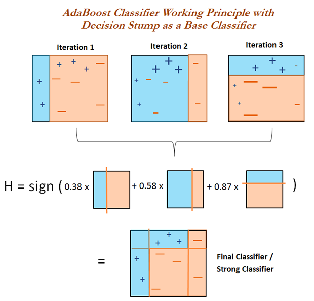
AdaBoost (Adaptive Boosting) is called adaptive boosting, and its main adaptive boosting is manifested in that the weights of the samples misclassified by the previous “individual learner” will increase, and the weights of the correctly classified samples will decrease, and they are used again to train the next basic classifier. In each round of iteration, a new weak classifier is added until a predetermined sufficiently small error rate is reached or the pre-specified maximum number of iterations is reached to determine the final strong classifier.
The difference between the AdaBoost algorithm and the Boosting algorithm is that it does not need to know the error of the weak classifier in advance, and the classification accuracy of the finally obtained strong classifier depends on the classification accuracy of all weak classifiers.
Adaboost algorithm process:
-
Data preparation: Obtain compliant data through data cleaning and data arrangement.
-
Initialize weights: If there are \(N\) training sample data, at the beginning, each data is given the same weight: \(1/N\).
-
Weak classifier prediction: Put the weighted training samples into the weak classifier for classification prediction.
-
Change weights: If a sample point is accurately classified, reduce its weight; if it is misclassified, then increase its weight. Then, the sample set with updated weights is used to train the next classifier.
-
Strong classifier combination: Repeat steps 3 and 4 until the training ends. Increase the weight of the weak classifier with a small classification error rate (the weight here is different from the sample weight), making it play a greater decisive role in the final classification function, and reduce the weight of the weak classifier with a large classification error rate, making it play a smaller decisive role in the final classification function, and finally output the result.
22.15. Model Building and Data Prediction#
After dividing the dataset, the next step is to build and predict the model. Next, we will implement it using scikit-learn.
AdaBoostClassifier(base_estimators,n_estimators)
Among them:
-
base_estimators: Represents the type of weak classifier, and the default is the CART classification tree. -
n_estimators: Represents the maximum number of weak learners, and the default value is50.
from sklearn.ensemble import AdaBoostClassifier

ad_model = AdaBoostClassifier(n_estimators=100)

ad_model.fit(X_train, y_train)
ad_y_pred = ad_model.predict(X_test)
ad_y_pred
array([3, 2, 3, 2, 0, 2, 3, 2, 3, 3, 3, 2, 1, 3, 3, 2, 2, 3, 1, 2, 1, 3,
       1, 3, 1, 2, 3, 3, 2, 3, 3, 3, 2, 2, 3, 3, 0, 1, 2, 2, 2, 1, 3, 3,
       1, 3, 3, 3, 3, 3, 3, 3, 0, 2, 3, 3, 1, 3, 2, 0, 3, 2, 0, 2, 2, 3,
       3, 3, 2, 3, 0, 3, 2, 2, 3, 2, 1, 2, 0, 2, 2, 1, 3, 3, 2, 3, 3, 1,
       3, 3, 1, 3, 3, 3, 2, 0, 2, 3, 0, 3, 1, 3, 1, 0, 3, 3, 3, 3, 2, 3,
       3, 1, 1, 1, 3, 3, 3, 3, 3])
accuracy_score(y_test, ad_y_pred) # 计算使用决策树预测的准确率
0.8151260504201681
From the results, it can be seen that the accuracy obtained by applying the Adaboost algorithm is not much different from that of the decision tree on this dataset.
22.16. Gradient Boosting Decision Tree (GBDT)#
Gradient Boosting Decision Tree (GBDT) is also a member of the Boosting algorithm family. Adaboost uses the error rate of the weak learner in the previous iteration to update the weights of the training set, while Gradient Boosting Decision Tree adopts the forward stagewise algorithm, and the weak learner is limited to using the CART tree model.
In the iteration of GBDT, assume that the strong learner obtained in the previous iteration is \(f_{t - 1}(x)\) and the loss function is \(L(y, f_{t - 1}(x))\). The goal of this round of iteration is to find a weak learner \(h_{t}(x)\) of the CART regression tree model such that the loss of this round \(L(y, f_{t}(x)) = L(y, f_{t - 1}(x) + h_{t}(x))\) is minimized. That is to say, in this round of iteration, finding the decision tree aims to minimize the loss of the samples as much as possible.
Algorithm process:
-
Data preparation: Obtain compliant data through data cleaning and data arrangement.
-
Initialize weights: If there are \(N\) training sample data, at the beginning, each data is assigned the same weight: \(1/N\).
-
Weak classifier prediction: Put the weighted training samples into the weak classifier for classification prediction.
-
CART tree fitting: Calculate the gradient value of each subsample, and fit a CART tree through the gradient value and the subsample.
-
Update the strong learner: Calculate the best fitting value through the loss function in the fitted CART tree, and update the previously composed strong learner.
-
Strong classifier combination: Repeat steps 3, 4, and 5 until the training ends, obtain a strong classifier, and finally output the result.
After dividing the dataset, the next step is to build and predict the model. Next, we will implement it using scikit-learn.
GradientBoostingClassifier(max_depth = 3, learning_rate = 0.1, n_estimators = 100, random_state = None)
Among them:
-
max_depth: Represents the maximum depth of the generated CART tree, with a default value of 3. -
learning_rate: Represents the learning efficiency, with a default value of 0.1. -
n_estimators: Represents the maximum number of weak learners, with a default value of 100. -
random_state: Represents the random number seed.
from sklearn.ensemble import GradientBoostingClassifier

gb_model = GradientBoostingClassifier(
    n_estimators=100, learning_rate=1.0, random_state=33
)

gb_model.fit(X_train, y_train)
gb_y_pred = gb_model.predict(X_test)
gb_y_pred
array([3, 0, 3, 2, 1, 2, 3, 2, 3, 3, 3, 2, 1, 3, 3, 2, 2, 0, 1, 2, 1, 1,
       1, 3, 3, 2, 3, 0, 3, 3, 3, 3, 2, 2, 3, 3, 0, 1, 2, 2, 2, 1, 3, 3,
       1, 3, 2, 3, 3, 3, 3, 3, 1, 2, 2, 0, 1, 3, 2, 3, 3, 2, 0, 2, 2, 3,
       2, 3, 2, 3, 0, 2, 2, 2, 3, 2, 1, 2, 0, 2, 2, 1, 3, 3, 0, 3, 3, 1,
       3, 3, 1, 3, 3, 3, 2, 0, 2, 3, 0, 3, 1, 3, 1, 1, 3, 3, 3, 3, 3, 3,
       3, 1, 1, 1, 3, 0, 3, 3, 3])
accuracy_score(y_test, gb_y_pred) # 计算使用决策树预测的准确率
0.8823529411764706
It can be seen that when using bagging and boosting algorithms, in most cases, better prediction results will be produced, but sometimes there may be unoptimized situations. In fact, this is the case for the selection of machine learning classifiers. There is no best classifier, only the most suitable one. Different datasets, due to their different data characteristics, perform differently among different classifiers.
22.17. Summary#
In this section of the experiment, we learned the principles of bagging and boosting algorithms in ensemble learning, and separately explained the representative algorithms in each category, namely Bagging Tree and Random Forest, as well as Adaboost and Gradient Boosting Tree. We also implemented the algorithms using scikit-learn.
Related Links