
15. Naive Bayes Implementation and Application#
15.1. Introduction#
In classification prediction, there are relatively few algorithms based on probability theory, and Naive Bayes is one of them. The Naive Bayes algorithm is simple to implement and highly efficient in predicting classifications, making it a very commonly used algorithm. This experiment mainly explains the principle of the Naive Bayes algorithm from two aspects: Bayes’ theorem and parameter estimation, and combines with data for implementation. Finally, a practical exercise is carried out through an example.
15.2. Key Points#
Conditional probability
Bayes’ theorem
Naive Bayes principle
Naive Bayes algorithm implementation
Maximum likelihood estimation
15.3. Basic Concepts#
The mathematical theory basis of Naive Bayes stems from probability theory. Therefore, before learning the Naive Bayes algorithm, a brief introduction to the probability theory knowledge involved in this experiment will be given first.
15.4. Conditional Probability#
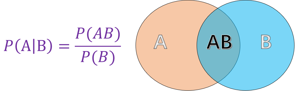
Conditional probability refers to the probability of event \(A\) given that another event \(B\) has already occurred. As shown in the figure:
Among them:
-
\(P(A)\) represents the probability of event \(A\) occurring.
-
\(P(B)\) represents the probability of event \(B\) occurring.
-
\(P(AB)\) represents the probability of events \(A\) and \(B\) occurring simultaneously.
And the finally calculated \(P(A|B)\) is the conditional probability, which represents the probability of event \(A\) occurring given that event \(B\) has occurred.
15.5. Bayes’ Theorem#
The basic concept of conditional probability was mentioned above. So, given the probability \(P(A|B)\) that event \(A\) occurs when event \(B\) is known to have occurred, how can we find \(P(B|A)\)? Bayes’ theorem comes into being. According to the conditional probability formula, we can get:
And similarly, through the conditional probability formula, we can get:
Substituting equation (2) into equation (1), we can obtain the complete Bayes’ theorem:
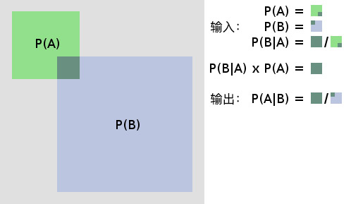
Next, through a diagram, we will comprehensively and vividly demonstrate the principles of conditional probability and Bayes’ theorem.
15.6. Prior Probability#
Prior Probability refers to the probability obtained based on past experience and analysis. For example, \(P(A)\) and \(P(B)\) in the above formula, or another example: Let \(X\) represent the probability of getting heads when flipping a fair coin. Obviously, based on our past experience, we would think that the probability of \(X\), \(P(X)=0.5\). Here, \(P(X) = 0.5\) is the prior probability.
15.7. Posterior Probability#
Posterior Probability is the reverse conditional probability obtained after an event occurs; that is, the reverse conditional probability obtained through Bayes’ formula based on the prior probability. For example, \(P(B|A)\) in the formula is the posterior probability obtained from the prior probabilities \(P(A)\) and \(P(B)\). Generally speaking, it is the “cause” in “seeking the cause from the result”.
15.8. Naive Bayes Principle#
Naive Bayes is an algorithm that combines Bayes’ principle and conditional independence. Its idea is very simple. According to Bayes’ formula:
The transformed expression is:
Equation (5) uses the prior probabilities, that is, the probabilities of features and categories; then uses the probability distributions of each feature in different categories, and finally calculates the posterior probability, that is, predicts different categories under the distributions of each feature.
Using the Bayesian principle to solve is固然 a good method, but in real life, there are interconnections between the features of the data. When calculating \(P(\text{Feature} \mid \text{Category})\), it is rather troublesome to consider the connections between the features. Naive Bayes, however, artificially separates each feature and assumes that the features are independent of each other.
The “naive” in Naive Bayes, that is, conditional independence, means that it assumes that all the attributes for prediction are independent of each other, and each attribute independently affects the classification result. Mathematically, conditional independence is expressed as: \(P(AB)=P(A) \times P(B)\). In this way, the Naive Bayes algorithm becomes simple, but sometimes it sacrifices a certain classification accuracy. For the predicted data, calculate the occurrence probabilities of each category when the attributes of the predicted data appear, and take the category with the largest probability value as the category of the predicted data.
Regarding Bayes’ theorem and the Naive Bayes method, here is an interesting video that hopefully helps everyone deepen their understanding.
15.9. Implementation of Naive Bayes Algorithm#
Previously, we mainly introduced several important probability theory knowledge in the Naive Bayes algorithm. Next, we will implement it specifically. The algorithm process is as follows:
-
Step 1: Let \(X = \{ a_{1},a_{2},a_{3},\ldots,a_{n} \}\) be the prediction data, where \(a_{i}\) is the feature value of the prediction data.
-
Step 2: Let \(Y = \{y_{1},y_{2},y_{3},\ldots,y_{m} \}\) be the set of categories.
-
Step 3: Calculate \(P(y_{1}\mid x)\), \(P(y_{2}\mid x)\), \(P(y_{3}\mid x)\), \(\ldots\), \(P(y_{m}\mid x)\).
-
Step 4: Find the maximum probability \(P(y_{k}\mid x)\) among \(P(y_{1}\mid x)\), \(P(y_{2}\mid x)\), \(P(y_{3}\mid x)\), \(\ldots\), \(P(y_{m}\mid x)\). Then \(x\) belongs to the category \(y_{k}\).
Next, we use Python to complete the classification of the Naive Bayes algorithm. First, generate a set of sample data: consisting of two categories, A and B, each category contains two feature values, x and y. Among them, the x feature contains three categories: r, g, b (red, green, blue), and the y feature contains three categories: s, m, l (small, medium, large), such as the data X = [g, l].
import pandas as pd


def create_data():
    # 生成示例数据
    data = {
        "x": [
            "r",
            "g",
            "r",
            "b",
            "g",
            "g",
            "r",
            "r",
            "b",
            "g",
            "g",
            "r",
            "b",
            "b",
            "g",
        ],
        "y": [
            "m",
            "s",
            "l",
            "s",
            "m",
            "s",
            "m",
            "s",
            "m",
            "l",
            "l",
            "s",
            "m",
            "m",
            "l",
        ],
        "labels": [
            "A",
            "A",
            "A",
            "A",
            "A",
            "A",
            "A",
            "A",
            "B",
            "B",
            "B",
            "B",
            "B",
            "B",
            "B",
        ],
    }
    data = pd.DataFrame(data, columns=["labels", "x", "y"])
    return data
After creating the data, the next step is to load the data and preview it.
data = create_data()
data
| labels | x | y | |
|---|---|---|---|
| 0 | A | r | m |
| 1 | A | g | s |
| 2 | A | r | l |
| 3 | A | b | s |
| 4 | A | g | m |
| 5 | A | g | s |
| 6 | A | r | m |
| 7 | A | r | s |
| 8 | B | b | m |
| 9 | B | g | l |
| 10 | B | g | l |
| 11 | B | r | s |
| 12 | B | b | m |
| 13 | B | b | m |
| 14 | B | g | l |
15.10. Parameter Estimation#
According to the principle of Naive Bayes, the decision factor for the final classification is to compare the magnitudes of \(\{P(\text{Category 1} \mid \text{Feature}), P(\text{Category 2} \mid \text{Feature}), \ldots, P(\text{Category } m \mid \text{Feature})\}\). According to Bayes’ formula, the denominator \(P(\text{Feature})\) for calculating each probability is the same. We only need to compare the magnitudes of the products of the numerators \(P(\text{Category})\) and \(P(\text{Feature} \mid \text{Category})\).
So how can we obtain \(P(\text{Category})\) and \(P(\text{Feature} \mid \text{Category})\)? In probability theory, the maximum likelihood estimation method and the Bayesian estimation method can be applied to estimate the corresponding probabilities.
15.11. Maximum Likelihood Estimation#
What is maximum likelihood? The following simple example will give you an intuitive understanding:
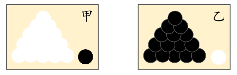
Prerequisites: Suppose there are two boxes with exactly the same appearance. Box A contains 99 white balls and 1 black ball; Box B contains 99 black balls and 1 white ball.
Question: When we conduct an experiment and take out a ball, and the result of the draw is a white ball. Then, may I ask from which box was the white ball taken?
I believe that your first impression is very likely that the white ball was taken from Box A. Because there are more white balls in Box A, this inference conforms to people’s experience. The “most likely” here is the “maximum likelihood”. The purpose of maximum likelihood estimation is to use the known sample results to reverse-infer the parameter values that are most likely to cause this result.
Maximum likelihood estimation provides a method for evaluating model parameters given observed data, that is, “the model is fixed, but the parameters are unknown”. Through a number of experiments, observe the results. If a certain parameter value can maximize the probability of the occurrence of the sample using the experimental results, it is called maximum likelihood estimation.
In probability theory, the method of solving maximum likelihood estimation is relatively complex. Based on experiments, we will explain how \(P(B)\) and \(P(B/A)\) are obtained through maximum likelihood estimation. \(P(\text{category})\) is expressed mathematically as:
In formula (6), \(y_{i}\) represents the category of the data, and \(c_{k}\) represents the category of each piece of data.
You can understand it in a popular way that in the existing training set, it is the proportion of each category in the total. For example, in the generated data, \(P(Y = A)=\frac{8}{15}\), which means there are 15 pieces of data in total in the training set, and 8 of them are of category \(A\).
Next, we use Python code to implement the solution of the prior probability \(P(\text{category})\):
def get_P_labels(labels):
    # P(\text{种类}) 先验概率计算
    labels = list(labels)  # 转换为 list 类型
    P_label = {}  # 设置空字典用于存入 label 的概率
    for label in labels:
        # 统计 label 标签在标签集中出现的次数再除以总长度
        P_label[label] = labels.count(label) / float(
            len(labels)
        )  # p = count(y) / count(Y)
    return P_label


P_labels = get_P_labels(data["labels"])
P_labels
{'A': 0.5333333333333333, 'B': 0.4666666666666667}
Since the formula for \(P(\text{feature} \mid \text{category})\) is rather cumbersome, it will not be presented here. It can be more clearly understood by simply using a narrative approach:
The actual prior estimate to be calculated is the probability of each category of the feature corresponding to each kind. For example, in the generated data, \(P(x_{1}=r \mid Y = A)=\frac{4}{8}\). There are 8 pieces of data of category \(A\), and among the data of category \(A\), 4 have the feature \(x\) being \(r\).
Similarly, we use code to implement the solution of the prior probability \(P(\text{feature} \mid \text{category})\). First, we merge the features by serial number to generate a NumPy array.
import numpy as np

# 将 data 中的属性切割出来,即 x 和 y 属性
train_data = np.array(data.iloc[:, 1:])
train_data
array([['r', 'm'],
       ['g', 's'],
       ['r', 'l'],
       ['b', 's'],
       ['g', 'm'],
       ['g', 's'],
       ['r', 'm'],
       ['r', 's'],
       ['b', 'm'],
       ['g', 'l'],
       ['g', 'l'],
       ['r', 's'],
       ['b', 'm'],
       ['b', 'm'],
       ['g', 'l']], dtype=object)
When looking for a certain feature belonging to a certain category, we use the method of comparing indexes to complete it. First, we get the indexes of each category:
labels = data["labels"]
label_index = []
# 遍历所有的标签,这里就是将标签为 A 和 B 的数据集分开,label_index 中存的是该数据的下标
for y in P_labels.keys():
    temp_index = []
    # enumerate 函数返回 Series 类型数的索引和值,其中 i 为索引,label 为值
    for i, label in enumerate(labels):
        if label == y:
            temp_index.append(i)
        else:
            pass
    label_index.append(temp_index)
label_index
[[0, 1, 2, 3, 4, 5, 6, 7], [8, 9, 10, 11, 12, 13, 14]]
Get the indexes of \(A\) and \(B\), where the first 8 pieces of data are of category \(A\) and the last 7 pieces of data are of category \(B\).
After obtaining the indexes of the categories, the next step is to find the index values of the feature \(r\) that we need.
# 遍历 train_data 中的第一列数据,提取出里面内容为r的数据
x_index = [
    i for i, feature in enumerate(train_data[:, 0]) if feature == "r"
]  # 效果等同于求类别索引中 for 循环

x_index
[0, 2, 6, 7, 11]
The result obtained is the data index value where the feature value of \(x\) is \(r\).
Finally, by comparing the index values of category \(A\), calculate the proportion of the data that meets both \(x = r\) and category \(A\) in category \(A\).
# 取集合 x_index (x 属性为 r 的数据集合)与集合 label_index[0](标签为 A 的数据集合)的交集
x_label = set(x_index) & set(label_index[0])
print("既符合 x = r 又是 A 类别的索引值:", x_label)
x_label_count = len(x_label)
# 这里就是用类别 A 中的属性 x 为 r 的数据个数除以类别 A 的总个数
print("先验概率 P(r|A):", x_label_count / float(len(label_index[0])))  # 先验概率的计算公式
既符合 x = r 又是 A 类别的索引值: {0, 2, 6, 7}
先验概率 P(r|A): 0.5
To facilitate the subsequent function calls, we integrate the code for calculating \(P(\text{feature} \mid \text{class})\) into a function.
def get_P_fea_lab(P_label, features, data):
    # P(\text{特征}∣种类) 先验概率计算
    # 该函数就是求 种类为 P_label 条件下特征为 features 的概率
    P_fea_lab = {}
    train_data = data.iloc[:, 1:]
    train_data = np.array(train_data)
    labels = data["labels"]
    # 遍历所有的标签
    for each_label in P_label.keys():
        # 上面代码的另一种写法,这里就是将标签为 A 和 B 的数据集分开,label_index 中存的是该数据的下标
        label_index = [i for i, label in enumerate(labels) if label == each_label]

        # 遍历该属性下的所有取值
        # 求出每种标签下,该属性取每种值的概率
        for j in range(len(features)):
            # 筛选出该属性下属性值为 features[j] 的数据
            feature_index = [
                i
                for i, feature in enumerate(train_data[:, j])
                if feature == features[j]
            ]

            # set(x_index)&set(y_index) 取交集,得到标签值为 each_label,属性值为 features[j] 的数据集合
            fea_lab_count = len(set(feature_index) & set(label_index))
            key = str(features[j]) + "|" + str(each_label)  # 拼接字符串

            # 计算先验概率
            # 计算 labels 为 each_label下,featurs 为 features[j] 的概率值
            P_fea_lab[key] = fea_lab_count / float(len(label_index))
    return P_fea_lab


features = ["r", "m"]
get_P_fea_lab(P_labels, features, data)
{'r|A': 0.5,
 'm|A': 0.375,
 'r|B': 0.14285714285714285,
 'm|B': 0.42857142857142855}
The prior probabilities under different categories can be obtained when the values of features \(x\) and \(y\) are \(r\) and \(m\) respectively.
15.12. Bayesian Estimation#
When doing maximum likelihood estimation, if some features are missing in a category, the probability value will be 0. At this time, it will affect the calculation result of the posterior probability and cause bias in classification. The best way to solve this problem is to use Bayesian estimation.
In the calculation of the prior probability \(P(\text{class})\), the mathematical expression of Bayesian estimation is:
Among them, \(\lambda \geq 0\) is equivalent to assigning a positive number to the frequency of each value of the random variable. When \(\lambda = 0\), it is the maximum likelihood estimation. Usually, \(\lambda = 1\) is taken, and this is called Laplace smoothing at this time. For example: in the generated data, \(P(Y = A)=\frac{8 + 1}{15+2*1}=\frac{9}{17}\). When \(\lambda = 1\), since there are two categories \(A\) and \(B\) in total, \(k\) takes 2.
Similarly, when calculating \(P(\text{feature} \mid \text{class})\), Laplace smoothing is also added to both the numerator and denominator in the calculation. For example: in the generated data, \(P(x_{1}=r \mid Y = A)=\frac{4 + 1}{8+3*1}=\frac{5}{11}\). Similarly, when \(\lambda = 1\), since there are three categories \(r\), \(g\), and \(b\) in \(x\), the value of \(k\) here is 3.
Through the above content, I believe you already have a certain impression of the principle of the Naive Bayes algorithm. Next, we will fully implement the Naive Bayes classification process. Among them, the parameter estimation method uses the maximum likelihood estimation.
def classify(data, features):
    # 朴素贝叶斯分类器
    # 求 labels 中每个 label 的先验概率
    labels = data["labels"]
    # 这里也就是求 P(B),P_label 为一个字典,存的是每个 B 对应的 P(B)
    P_label = get_P_labels(labels)
    P_fea_lab = get_P_fea_lab(P_label, features, data)  # 这里是在求 P(A|B)

    P = {}
    P_show = {}  # 后验概率
    for each_label in P_label:
        P[each_label] = P_label[each_label]
        # 遍历每个标签下的每种属性
        for each_feature in features:
            # 拼接字符串为 P(B/A) 用于字典的键值
            key = str(each_label) + "|" + str(features)
            # 计算 P(B/A) = P(B) * P(A/B) 因为所有的后验概率,分母相同。因此,在计算时可以忽略掉。
            P_show[key] = (
                P[each_label] * P_fea_lab[str(each_feature) + "|" + str(each_label)]
            )
            # 把刚才算的概率放到 P 列表里面,这个 P 列表的键值变成了标签。
            # 这样做的目的,其实是为了在后面取最大时,取出就是标签,而不是 标签|特征
            P[each_label] = (
                P[each_label] * P_fea_lab[str(each_feature) + "|" + str(each_label)]
            )
    # 输出 P_show 和 P 观察,发现他们的概率值没有变,只是字典的 key 值变了
    print(P_show)
    print(P)
    features_label = max(P, key=P.get)  # 概率最大值对应的类别
    return features_label
classify(data, ["r", "m"])
{"A|['r', 'm']": 0.1, "B|['r', 'm']": 0.02857142857142857}
{'A': 0.1, 'B': 0.02857142857142857}
'A'
For the data with features \([r,m]\), the probability values of different classes are obtained through Naive Bayes classification. After comparison, it is classified into class \(A\).
15.13. Three Common Models of Naive Bayes#
After understanding the principle of the Naive Bayes algorithm, in actual data, we can divide the Naive Bayes model according to the different data types of features when calculating the prior probability, and it can be divided into: the multinomial model, the Bernoulli model, and the Gaussian model.
15.14. Multinomial Model#
When the feature values are discrete, the multinomial model is often used. In fact, in the parameter estimation of the above experiments, the multinomial model we applied is exactly this one. To avoid the situation where the probability value is 0, the multinomial model uses Bayesian estimation.
15.15. Bernoulli Model#
Like the multinomial model, the Bernoulli model is applicable to the case of discrete features. The difference is that in the Bernoulli model, the value of each feature can only be 1 and 0 (taking text classification as an example, if a certain word appears in a document, its feature value is 1, otherwise it is 0).
In the Bernoulli model, the conditional probability \(P(x_{i} \mid y_{k})\) is calculated as follows:
-
When the feature value \(x_{i}=1\), \(P(x_{i} \mid y_{k})=P(x_{i}=1 \mid y_{k})\);
-
When the feature value \(x_{i}=0\), \(P(x_{i} \mid y_{k})=P(x_{i}=0 \mid y_{k})\).
15.16. Gaussian Model#
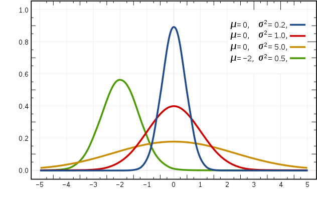
When the features are continuous variables, without smoothing, using the multinomial model will result in many \(P(x_{i} \mid y_{k}) = 0\). In this case, even with smoothing, the resulting conditional probabilities are difficult to describe the real situation. Therefore, when dealing with continuous feature variables, the Gaussian model is adopted. The Gaussian model assumes that the feature data of continuous variables follows a Gaussian distribution. The expression of the Gaussian distribution function is:
where:
-
\(\mu_{y_{k},i}\) represents the mean of the \(i\)-th feature in the samples of class \(y_{k}\).
-
\(\sigma ^{2}_{y_{k},i}\) represents the variance of the \(i\)-th feature in the samples of class \(y_{k}\).
The schematic diagram of the Gaussian distribution is as follows:
15.17. Naive Bayes Spam Classification#
Next, we apply the Naive Bayes algorithm model to classify and predict real data. Spam filtering is a very classic problem in machine learning, which involves the operation of classifying emails into spam or ham. The spam folder in your Gmail account is the best example.
15.18. Dataset Introduction and Preprocessing#
First, let’s get to know the dataset used in this experiment: trec06c.
trec06c is a publicly available spam corpus provided by the Text REtrieval Conference (TREC). It is divided into an English dataset (trec06p) and a Chinese dataset (trec06c). The emails contained in it are sourced from real emails, retaining the original format and content of the emails.
You can go to
2006 TREC Public Spam Corpora
to download the file
trec06c.tgz, or you can also use the mirror link to download:
wget -nc "https://cdn.aibydoing.com/aibydoing/files/trec06c.zip"  # 下载数据
unzip -o trec06c.zip
Next, we use
read_table
to load the dataset.
data = pd.read_table('trec06c/full/index', header=None,
                     encoding='gb2312', delim_whitespace=True)
data.head()
| 0 | 1 | |
|---|---|---|
| 0 | spam | ../data/000/000 |
| 1 | ham | ../data/000/001 |
| 2 | spam | ../data/000/002 |
| 3 | spam | ../data/000/003 |
| 4 | spam | ../data/000/004 |
After reading, it can be seen that there are a total of
64,620
samples in the entire dataset. The first column represents
whether it is spam. The label
spam
indicates spam, and the label
ham
indicates normal emails. The second column is the path to
the text file of the email content.
Next, replace
spam
with
0
and
ham
with
1, and then replace the file paths. To speed up the
operation, only 10,000 sample data are used in this
experiment.
df = data.replace(['spam', 'ham'], [0, 1])  # 0 替代 spam,1 替代 ham
df = df.replace(regex=["\.."], value='trec06c')  # 替换掉文件路径
df = df.sample(len(df), random_state=1, )[:10000]  # 打乱样本并取前 1 万条数据
df.groupby(0).count()  # 统计样本
| 1 | |
|---|---|
| 0 | |
| 0 | 6595 |
| 1 | 3405 |
After counting the sample size, there are 6,595 spam emails and 3,405 normal emails.
You can use shell commands to output the content of a spam email, but you need to convert the encoding to display Chinese properly.
!cat "trec06c/data/000/002" | iconv -f GBK -t UTF-8 # 显示文件内容并转为 UTF-8 编码
Received: from 163.con ([61.141.165.252])
	by spam-gw.ccert.edu.cn (MIMEDefang) with ESMTP id j7CHJ2B9028021
	for <[email protected]>; Sun, 14 Aug 2005 10:04:03 +0800 (CST)
Message-ID: <[email protected]>
From: =?GB2312?B?1cW6o8TP?= <[email protected]>
Subject: =?gb2312?B?uavLvtK1zvEutPq/qreixrGjoQ==?=
To: [email protected]
Content-Type: text/plain;charset="GB2312"
Date: Sun, 14 Aug 2005 10:17:57 +0800
X-Priority: 2
X-Mailer: Microsoft Outlook Express 5.50.4133.2400

尊敬的贵公司(财务/经理)负责人您好!
        我是深圳金海实业有限公司(广州。东莞)等省市有分公司。
    我司有良好的社会关系和实力,因每月进项多出项少现有一部分
    发票可优惠对外代开税率较低,增值税发票为5%其它国税.地税.
    运输.广告等普通发票为1.5%的税点,还可以根据数目大小来衡
    量优惠的多少,希望贵公司.商家等来电商谈欢迎合作。

       本公司郑重承诺所用票据可到税务局验证或抵扣!
    欢迎来电进一步商谈。
    电话:13826556538(24小时服务)
    信箱:[email protected]
    联系人:张海南


       顺祝商祺


                   深圳市金海实业有限公司
An email consists of two parts. The first part contains
information about the email, such as the sender, subject,
etc., and the second part is the body of the email. These
files are not encoded in
UTF-8, so they need to be converted to
UTF-8
encoding.
Since only the content of the email body will be used in this experiment, the first part needs to be removed. Additionally, there are many other unnecessary contents such as links in the body part. Therefore, we need to perform some data preprocessing on the original data, including the following contents.
-
Convert the encoding format of the source data to
UTF-8format. -
Filter characters: Remove all non-Chinese characters, such as punctuation marks, English characters, numbers, website links and other special characters.
Filter stop words.
-
Perform word segmentation on the email content.
In the steps of data cleaning, first, all English, numbers,
punctuation marks, and special symbols were filtered out
through regular expressions, and finally only Chinese
characters were retained. At the same time, there were still
some strange-looking characters in the content, which were
filtered by the Unicode Chinese encoding range
0x4e00-0x9fff.
import re

def clean_str(line):
    # 清理邮件,替换不需要的字符串
    line.strip('\n')
    line = re.sub(r"[^\u4e00-\u9fff]", "", line)
    line = re.sub(
        "[0-9a-zA-Z\-\s+\.\!\/_,$%^*\(\)\+(+\"\')]+|[+——!,。?、~@#¥%……&*()<>\[\]::★◆【】《》;;=??]+", "", line)
    return line.strip()
After completing the initial cleaning of the email text, the next step is to perform word segmentation on the text. In the experiment, we used the very famous Jieba module.
In Chinese, there are many non-content words or other words
that have no actual function. These words must be filtered
after word segmentation, and this step is to filter stop
words. By downloading a pre-set stop word list and then
judging whether a word is a stop word to filter the word
segmentation results. The course provides a relatively
comprehensive
stopwords.txt
file, which needs to be downloaded before it can be used.
Additionally, if it is a blank line, it needs to be removed.
After word segmentation, all results with only one character
need to be removed, which is easy to understand because a
single character basically has no content.
# 下载停用词表
wget -nc "https://cdn.aibydoing.com/aibydoing/files/stopwords.txt"
文件 “stopwords.txt” 已经存在;不获取。
Then, according to the logic stated above, write functions for word segmentation and stop word filtering.
def load_stopwords(file_path):
    # 加载停用词
    with open(file_path, 'r') as f:
        stopwords = [line.strip('\n') for line in f.readlines()]
    return stopwords

stopwords = load_stopwords('stopwords.txt')
stopwords
import jieba

def process(file_path, test_mode=False):
    # 清洗一封邮件
    '''
    - file_path: 文本文件路径
    - test_mode: 测试模式,后文我们会将一个字符串写入文件(utf-8 编码),而训练文件以 GBK 编码,
                 如果自己实现分类,请注意编码格式,通常为 utf-8
    - return: words, 处理、分词之后的有效词语
    '''
    words = []
    with open(file_path, 'rb') as f:
        for line in f.readlines():
            if not test_mode:
                line = line.strip().decode("gbk", 'ignore')
            else:
                line = line.strip().decode("utf-8", 'ignore')
            line = clean_str(line)
            if len(line) == 0:
                continue
            seg_list = list(jieba.cut(line, cut_all=False))
            for x in seg_list:
                if len(x) <= 1:
                    continue
                if x in stopwords:
                    continue
                words.append(x)
    return words
Next, we attempt to perform word segmentation and stop word
filtering on the spam emails in
trec06c/data/000/000.
words = process('trec06c/data/000/000')
" ".join(words)
'上海 培训 课程 财务 纠淼 沙盘 模拟 财务 课程 背景 一位 管理 技术人员 懂得 技术 角度 衡量 合算 方案 也许 却是 财务 陷阱 表面 赢利 亏损 使经 营者 接受 技术手段 财务 运作 相结合 每位 管理 技术人员 老板 角度 思考 规避 财务 陷阱 管理决策 目标 一致性 课程 沙盘 模拟 案例 分析 企业 管理 技术人员 财务管理 知识 利用 财务 信息 改进 管理决策 管理 效益 最大化 学习 课程 会计 财务管理 提高 日常 管理 活动 财务 可行性 业绩 评价 方法 评估 业绩 实施 科学 业绩考核 合乎 财务 墓芾 老板 思维 同步 分析 关键 业绩 指标 战略规划 预算 企业 管理 重心 管理 系统性 课程 大纲 财务 工作 内容 作用 财务会计 财务 专家 思维 模式 财务 工作 内容 管理者 利用 财务 管理 决策 阅读 分析 财务报表 会计报表 损益表 阅读 分析 资产 负债表 阅读 分析 资金 流量 现金流量 阅读 分析 会计报表 之间 关系 会计报表 读懂 企业 状况 案例 分析 报表 判断 企业 业绩 水平 财务 手段 成本 控制 产品成本 概念 本浚利 分析 标准 成本 制度 成本 控制 作用 目标 成本法 控制 产品成本 保证 利润 水平 作业 成本法 管理 分析 实施 精细 成本 管理 沉没 成本 机会成本 正确 决策 改善 采购 生产 环节 运作 改良 企业 整体 财务状况 综合 案例 分析 财务 尚械 墓芾 醴桨 管理 技术 方案 可行性 分析 产品开发 财务 可行性 分析 产品 增产 减产 财务 可行性 分析 生产 设备 改造 更新 决策分析 投资 项目 现金流 分析 投资 项目 评价 方法 现值 法分析 资金 时间 价值 分析 综合 案例 演练 公司 费用 控制 公司 费用 控制 费用 方法 影响 费用 因素 分析 成本 中心 费用 控制 利润 中心 业绩考核 投资 中心 业绩 评价 利用 财务 数据分析 改善 绩效 公司财务 分析 核心 思路 关键 财务指标 解析 盈利 能力 分析 资产 回报率 股东权益 回报率 资产 流动 速率 风险 指数 分析 流动比率 负债 权益 比率 营运 偿债 能力 财务报表 综合 解读 综合 财务 信息 透视 公司 运作 水平 案例 分析 上市公司 财务状况 分析 评价 企业 运营 管理 沙盘 模拟 模拟 体验式 教学 小组 模拟 公司 生产 销售 财务 分析 过程 钥怪 邢嗷逖 企业 乐趣 讲师 学员 分享 解决问题 模型 工具 学员 身同 转化 导师 简介 管理 工程硕士 高级 炯檬 国际 职业 培训师 认证 职业 培训师 历任 跨国公司 生产 负责人 工业 工程 管理 会计 分析师 营运 总监 高级 管理 职务 多年 担任 价值 工程 审稿人 辽宁省 营口市 商业银行 独立 职务 企业 管理 研究 王老师 技术 成本 控制 管理 会计 决策 课程 讲授 松下 可口可乐 康师傅 果汁 雪津 啤酒 吉百利 食品 冠捷 电子 明达 塑胶 正新 橡胶 美国 集团 广上 科技 美的 空调 中兴通讯 京信 通信 联想 电脑 材料 中国 公司 艾克森 金山 石化 中国 化工 进出口 公司 正大 集团 大福 饲料 厦华 集团 灿坤 股份 东金 电子 太原 钢铁集团 深圳 开发 科技 大冷 运输 制冷 三洋 华强 名企 提供 项目 辅导 专题 培训 王老师 授课 狙榉 风格 幽默诙谐 逻辑 清晰 过程 互动 案例 生动 深受 学员 喜爱 授课 时间 地点 周六日 上海 课程 费用 元人 包含 培训 费用 午餐 证书 资料 优惠 三人 参加 赠送 名额 联系人 电话传真'
Then, we need to perform word segmentation on all samples. Since this process takes a long time to execute, the tqdm module is used here to display the processing progress.
from tqdm import tqdm

tqdm.pandas()  # 使用 tqdm 显示进度
# 将 apply 函数替换为 progress_apply 以使用 tqdm 显示处理进度
df["words"] = df[1].progress_apply(process)
df.head()
| 0 | 1 | words | |
|---|---|---|---|
| 37029 | 1 | trec06c/data/123/129 | [恋爱, 第三次, 告诉, 再见面, 时间, 我要, 考研, 考到, 北京, 是否是, 喜欢... |
| 2257 | 0 | trec06c/data/007/157 | [欣欣, 签约, 推出, 中国, 第一个, 彩铃, 歌手, 稀稀, 龙乐, 公司, 签约, ... |
| 50881 | 1 | trec06c/data/169/181 | [男生, 思路, 简单, 心痛, 直说, 原因, 不让, 担心, 他累, 不去, 撒娇, 撒... |
| 10843 | 0 | trec06c/data/036/043 | [] |
| 4689 | 0 | trec06c/data/015/189 | [本港, 会计师, 权威机构, 香港, 瑞丰, 会计师, 事务所, 注册, 海外, 国际, ... |
After word segmentation, we need to further process the word segmentation results. Since words cannot be directly understood by algorithms, we need to encode the word segmentation results into vectors that can be input into the algorithms here. Here, we will use the commonly used Word2vec method in the field of natural language. This method was created by Google and you can read about it at Word2vec - Wikipedia.
Since Google only provides the C version of the Word2vec method, the experiment uses the Word2vec API provided by gensim. This process takes a long time to execute, please be patient.
from gensim.models import Word2Vec
from tqdm import tqdm_notebook

# 移除一些不必要的警告
import warnings

warnings.filterwarnings("ignore")

# 导入上面保存的分词数组
data = df["words"]

# 训练 Word2Vec 浅层神经网络模型
w2v_model = Word2Vec(vector_size=100, min_count=10)
w2v_model.build_vocab(data)
w2v_model.train(data, total_examples=w2v_model.corpus_count, epochs=5)
w2v_model
<gensim.models.word2vec.Word2Vec at 0x168950fd0>
def sum_vec(text):
    # 对每个句子的进行词向量求和计算
    vec = np.zeros(100).reshape((1, 100))
    for word in text:
        try:
            # 得到句子中每个词的词向量并累加在一起
            vec += w2v_model.wv.get_vector(word).reshape((1, 100))
        except KeyError:
            continue
    return vec
# 将词向量保存为 Ndarray
data_vec = np.concatenate([sum_vec(z) for z in tqdm_notebook(data)])
data_vec.shape
(10000, 100)
In the code, we initialize a
\((1, 100)\)
vector filled with all zeros as a container. We loop through
an article
text
and use
w2v_model.wv.get_vector()
to output the vector representation of each word in the
pre-trained model
w2v_model. Then, we accumulate the vector representations of each
word using
vec
to obtain the overall vector representation of the article
text.
You will find that the word segmentation results of the emails have been converted into vectors. \((10000, 100)\) indicates that there are 10,000 samples, and the email content has been encoded into vectors of a specified length of 100.
Next, we can start splitting the data and using Naive Bayes for modeling.
15.19. Data Splitting and Modeling#
After data preprocessing, we also need to split the dataset
into a training set and a test set. According to experience,
the training set accounts for 80% and the test set accounts
for 20%. Here, we also use the
train_test_split
function in the scikit-learn module to complete the dataset
splitting.
from sklearn.model_selection import train_test_split

feature_data = data_vec
label_data = df[0].values
# 分割数据
X_train, X_test, y_train, y_test = train_test_split(
    feature_data, label_data, test_size=0.2, random_state=4
)

X_train.shape, X_test.shape, y_train.shape, y_test.shape
((8000, 100), (2000, 100), (8000,), (2000,))
In the previous experiment, we implemented the Naive Bayes algorithm using Python. Now, we will implement it using scikit-learn. Since the polynomial model in scikit-learn requires the input matrix to be non-negative, we use the Bernoulli model here. The scikit-learn Naive Bayes Bernoulli model class and its parameters are as follows:
sklearn.naive_bayes.BernoulliNB(alpha=1.0, binarize=0.0, fit_prior=True, class_prior=None)
Among them:
-
alpharepresents the smoothing parameter. For Laplace smoothing,alpha = 1. -
fit_priorindicates whether to use prior probabilities, with the default beingTrue. -
class_priorrepresents the prior probabilities of the classes.
Common methods:
-
fit(x,
                          y)
selects a suitable Bayesian classifier. -
predict(X)makes predictions on the dataset and returns the prediction results.
from sklearn.naive_bayes import BernoulliNB

model = BernoulliNB()  # 定义伯努利模型分类器
model.fit(X_train, y_train)  # 模型训练
y_pred = model.predict(X_test)  # 模型预测
y_pred
array([0, 0, 1, ..., 0, 0, 0])
After we train the model and perform classification predictions, we can obtain the prediction accuracy by comparing the prediction results with the true results.
from sklearn.metrics import accuracy_score

accuracy_score(y_test, y_pred)
0.9435
It can be seen that by using the Naive Bayes algorithm for classification, an accuracy rate of 95% can be obtained, and the effect is quite good.
15.20. Summary#
This section of the experiment starts from the relevant concepts of probability theory and expounds the core theorem of the Naive Bayes algorithm, namely Bayes’ theorem. At the same time, the experiment explains the principle and implementation process of the Naive Bayes algorithm by combining theory with code. It should be noted that the knowledge points of probability theory involved in the Naive Bayes algorithm are prone to confusion, and it is recommended to distinguish them by combining actual examples.