
11. Logistic Regression Implementation and Application#
11.1. Introduction#
Logistic Regression, also known as Logit Regression, is a very basic classification method in machine learning. Due to its simplicity and efficiency, it has been widely applied in practical scenarios. In this experiment, we will explore the principle and algorithm implementation of Logistic Regression and use scikit-learn to build a Logistic Regression classification prediction model.
11.2. Key Points#
Linearly separable and inseparable
Sigmoid distribution function
Logistic regression model
Logarithmic loss function
Gradient descent method
Logistic Regression, when you hear this name, I believe the first thing you notice is “Regression”. We have learned Linear Regression before, so what are the differences and connections between Logistic Regression and it?
However, it needs to be emphasized at the beginning of this experiment: Logistic Regression is a classification method, not a regression method. You need to firmly remember this and not get confused. So, why does Logistic Regression have a name with the word “Regression”? Does it really have nothing to do with the regression method mentioned before?
Regarding this question, after learning all the content of this experiment, I believe you will get the answer.
11.3. Linearly separable and inseparable#
First of all, we need to get in touch with a concept, that is, linearly separable. As shown in the following figure, in a two-dimensional plane, if the samples can be separated by only one straight line, it is called linearly separable, otherwise it is linearly inseparable.

Of course, in three-dimensional space, if the samples can be separated by a plane, it is also called linearly separable. Since this experiment will not cover it, we will not go into it in depth here.
11.4. Using Linear Regression for Classification#
In the previous experiments, we focused on learning linear regression. Briefly summarized, linear regression is to predict more continuous values by fitting a straight line. In fact, in addition to regression problems, linear regression can also be used to handle classification problems in special cases. For example:
If we have the following dataset, this dataset contains only 1 feature and 1 target value. For example, we count the scores of students in a certain course and determine whether they PASS the course based on the learning duration.
scores = [
    [1],
    [1],
    [2],
    [2],
    [3],
    [3],
    [3],
    [4],
    [4],
    [5],
    [6],
    [6],
    [7],
    [7],
    [8],
    [8],
    [8],
    [9],
    [9],
    [10],
]
passed = [0, 0, 0, 0, 0, 0, 0, 0, 0, 0, 1, 0, 0, 1, 1, 1, 1, 1, 1, 1]
In the above dataset, the values of
passed
are only 0 and 1, which are numerical data. However, here we
represent 0 and 1 as “passed” and “not passed” respectively,
then it is converted into a classification problem.
Moreover, this is a typical binary classification problem.
Binary classification means there are only two categories,
and it can also be called: 0-1 classification problem.
For such a binary classification problem, how can we use linear regression to solve it?
Here, we can define that the result
\(f(x)>0.5\)
(close to 1) calculated by the linear fitting function
\(f(x)\)
represents
PASS, while
\(f(x)\leq0.5\)
(close to 0) represents not passing.
In this way, we can cleverly use linear regression to solve the binary classification problem.
Next, let’s start with the practical content. First, draw a scatter plot of the dataset corresponding to the two-dimensional plane.
from matplotlib import pyplot as plt

%matplotlib inline

plt.scatter(scores, passed, color="r")
plt.xlabel("scores")
plt.ylabel("passed")
Text(0, 0.5, 'passed')

Then, we use scikit-learn to complete the process of linear regression fitting. I believe that after learning the previous content, you should be very familiar with the process of linear regression fitting.
from sklearn.linear_model import LinearRegression

model = LinearRegression()
model.fit(scores, passed)
model.coef_, model.intercept_
(array([0.1446863]), -0.36683738796414866)
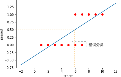
Next, plot the fitted line onto the scatter plot.
import numpy as np

x = np.linspace(-2, 12, 100)

plt.plot(x, model.coef_[0] * x + model.intercept_)
plt.scatter(scores, passed, color="r")
plt.xlabel("scores")
plt.ylabel("passed")
Text(0, 0.5, 'passed')

If according to the above definition, that is, the result
\(f(x)\)
calculated by the linear fitting function
\(f(x)>0.5\)
represents
PASS, while
\(f(x)\leq0.5\)
represents not passing.
Then, as shown in the figure below, all parts where
scores
are greater than the
\(x\)-coordinate value corresponding to the orange vertical line
will be judged as
PASS, that is, the
2
points circled by the brown selection box are misclassified.
11.5. Sigmoid Distribution Function#
In the above content, although we can use linear regression to solve binary classification problems, its results are not ideal. Especially in the \(0 - 1\) classification problem, linear regression may also produce negative values or numbers greater than \(1\) during the calculation process. Therefore, in today’s experiment, we can use a method called logistic regression to better complete the \(0 - 1\) classification problem.
Here, we need to first come into contact with a function called Sigmoid, and the definition of this function is as follows:
You may feel a bit confused. Why do we suddenly introduce such a function? Next, let’s plot the curve of this function and you may understand.
def sigmoid(z):
    sigmoid = 1 / (1 + np.exp(-z))
    return sigmoid
z = np.linspace(-12, 12, 100)  # 生成等间距 x 值方便绘图
plt.plot(z, sigmoid(z))
plt.xlabel("z")
plt.ylabel("y")
Text(0, 0.5, 'y')

The above figure is the graph of the Sigmoid function. You will be surprised to find that this graph呈现出完美的 S 型(呈现出完美的 S 型(the meaning of Sigmoid)). Its value only ranges between 0 and 1, and it is symmetric about the z = 0 axis. At the same time, when z is larger, y is closer to 1, and when z is smaller, y is closer to 0. If we take 0.5 as the dividing point and classify the values > 0.5 or < 0.5 into two categories, isn’t this the perfect choice for solving the 0 - 1 binary classification problem?
11.6. Logistic Regression Model#
In the previous example, the experiment used linear regression to solve the classification problem. It was found that the y-values of the fitted linear function were between \((-\infty, +\infty)\). The Sigmoid function was mentioned, and its y-values are between \((0, 1)\).
Here, we need to introduce another mathematical definition. That is, if a set of continuous random variables conforms to the sample distribution of the Sigmoid function, it is called a logistic distribution. The logistic distribution is a theorem in probability theory and is a continuous probability distribution.
Then, here we consider combining the two, that is, compressing the result of the linear function fitting to the range between \((0, 1)\) using the Sigmoid function. If the y-value of the linear function is larger, it means the probability is closer to 1, and vice versa, closer to 0.
Therefore, in logistic regression, it is defined that:
In Equation (3), we multiply each feature \(x\) by the coefficient \(w\), and then calculate the value of \(f(z)\) through the Sigmoid function to obtain the probability. Among them, \(z\) can be regarded as the classification boundary. Therefore:
Since the target value \(y\) has only two values, 0 and 1, if we denote the probability of \(y = 1\) as \(h_{w}(x)\), then the probability of \(y = 0\) at this time is \(1 - h_{w}(x)\). Then, we can denote the conditional probability distribution of the logistic regression model as:
The above Equation (5) is not convenient for calculation and can be equivalently written as the likelihood function:
You can verify that the meaning of Equation (6) is that when \(y = 1\), the probability is \(h_{w}(x)\), and when \(y = 0\), the probability is \(1 - h_{w}(x)\).
Above, we just took one sample as an example. For the total probability of \(i\) samples, it can actually be regarded as the product of the probabilities of single samples, denoted as \(L(w)\):
Since expressing the product is very complex, we apply a mathematical technique, that is, taking the logarithm on both sides to convert the product into a sum form, namely:
11.7. Logarithmic Loss Function#
In fact, formula (8) is called the log-likelihood function, which measures the total probability of an event occurring. According to the principle of maximum likelihood estimation, we only need to find the maximum value of \(L(w)\) to obtain the estimated value of \(w\). In machine learning problems, we need a loss function and optimize the parameters by finding its minimum value. Therefore, taking the negative of the log-likelihood function can be used as the logarithmic loss function for logistic regression:
To measure the average loss over the entire dataset, formula (9) takes the average over all samples to form the final logarithmic loss function for logistic regression. At this point, you might wonder why logistic regression doesn’t use the squared loss function in linear regression?
This actually has a mathematical basis. The purpose of setting the loss function is to find the minimum value of the loss function through optimization methods next. The minimum loss means the optimal model. In optimization solving, only convex functions (https://zh.wikipedia.org/zh-hans/凸函数) can often obtain the global minimum, while non-convex functions often get local optima. However, when the squared loss function is used for logistic regression solving, a non-convex function is obtained, that is, the global optimum cannot be obtained in most cases. Using the logarithmic loss function here avoids this problem.

In the non-convex function shown above, there are a global minimum and local minima.
Of course, the above statement involves a lot of mathematical knowledge. Especially something like optimization theory, which is only covered in graduate courses and can be a bit difficult to understand. If you can’t understand it, just remember that in logistic regression, we use the logarithmic loss function.
Next, we implement formula (9) with code:
def loss(h, y):
    loss = (-y * np.log(h) - (1 - y) * np.log(1 - h)).mean()
    return loss
11.8. Gradient Descent#
Above, we have successfully defined and implemented the logarithmic loss function. So, now we are only one step away from solving for the optimal parameters, which is to find the minimum value of the loss function.
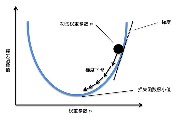
To find the minimum value of formula (9), a solution method called “gradient descent” is introduced here. Gradient descent is a very commonly used and classic optimization algorithm, and through this method, we can quickly find the minimum value of a function. The principle of gradient descent will be explained below. I hope you can understand it carefully, as gradient descent will be used in many subsequent contents.
To understand gradient descent, first, we need to be clear about what “gradient” is. The gradient is a vector, which represents that the directional derivative of a certain function at that point reaches the maximum along this direction, that is, the function changes fastest at that point along this direction (the direction of this gradient), and the rate of change is the largest (the magnitude of this gradient). In short, for a univariate function, the gradient refers to the derivative at a certain point. For a multivariate function, the gradient refers to the vector composed of the partial derivatives at a certain point.
Since the function changes fastest along the gradient direction, the core of the “gradient descent method” is that we search for the minimum value of the loss function (the opposite direction of the gradient) along the direction of gradient descent. The process is shown in the following figure.
Therefore, we take the partial derivatives of formula (9) to obtain the gradient. However, formula (9) is relatively complex now, so we first simplify formula (9). Let’s first look at \(\log (h_{w}(x^{(i)}))\). Combining with formula (4), we get:
Similarly, let’s look at \(\log(1 - h_{w}(x^{(i)}))\):
Substitute formulas (10) and (11) into formula (9) and simplify to get:
Now, take the derivative of formula (12) to get:
Substitute formula (4) into formula (13) to get:
For ease of understanding, express formula (14) in vector form as:
When we obtain the direction of the gradient and then multiply it by a constant \(\alpha\), we can get the step size of each gradient descent (the length of the arrow in the above figure). Finally, through multiple iterations, we find the point where the gradient change is very small, which corresponds to the minimum value of the loss function. Among them, the constant \(\alpha\) is often also called the learning rate. The process of performing weight updates is as follows:
Next, we implement formula (15) in code:
def gradient(X, h, y):
    gradient = np.dot(X.T, (h - y)) / y.shape[0]
    return gradient
11.9. Logistic Regression Python Implementation#
So far in the experiment, we already have the basic elements
for implementing logistic regression. Next, we will use
logistic regression to complete a classification task with a
set of sample data. First, download and load the sample
data. The name of the dataset is:
course-8-data.csv.
wget -nc https://cdn.aibydoing.com/aibydoing/files/course-8-data.csv
import pandas as pd

df = pd.read_csv("course-8-data.csv", header=0,)  # 加载数据集
df.head()  # 预览前 5 行数据
| X0 | X1 | Y | |
|---|---|---|---|
| 0 | 5.1 | 3.5 | 0 |
| 1 | 4.9 | 3.0 | 0 |
| 2 | 4.7 | 3.2 | 0 |
| 3 | 4.6 | 3.1 | 0 |
| 4 | 5.0 | 3.6 | 0 |
As can be seen, this dataset has two feature variables X0 and X1, and one target value Y. Among them, the target value Y only contains 0 and 1, which is a typical 0-1 classification problem. We try to plot this dataset to see the data distribution.
plt.figure(figsize=(10, 6))
plt.scatter(df["X0"], df["X1"], c=df["Y"])
<matplotlib.collections.PathCollection at 0x17b830d00>

In the figure above, dark blue represents 0 and yellow represents 1. Next, we will use logistic regression to complete the classification of the two types of data. That is, the linear function in formula (3).
For the convenience of code display, the code for the logistic regression model, loss function, and gradient descent mentioned above is presented together here. Next, the code for implementing logistic regression using Python will be shown.
def sigmoid(z):
    # Sigmoid 分布函数
    sigmoid = 1 / (1 + np.exp(-z))
    return sigmoid


def loss(h, y):
    # 损失函数
    loss = (-y * np.log(h) - (1 - y) * np.log(1 - h)).mean()
    return loss


def gradient(X, h, y):
    # 梯度计算
    gradient = np.dot(X.T, (h - y)) / y.shape[0]
    return gradient


def Logistic_Regression(x, y, lr, num_iter):
    # 逻辑回归过程
    intercept = np.ones((x.shape[0], 1))  # 初始化截距为 1
    x = np.concatenate((intercept, x), axis=1)
    w = np.zeros(x.shape[1])  # 初始化参数为 0

    for i in range(num_iter):  # 梯度下降迭代
        z = np.dot(x, w)  # 线性函数
        h = sigmoid(z)  # sigmoid 函数

        g = gradient(x, h, y)  # 计算梯度
        w -= lr * g  # 通过学习率 lr 计算步长并执行梯度下降

        l = loss(h, y)  # 计算损失函数值

    return l, w  # 返回迭代后的梯度和参数
Then, we set the learning rate and the number of iterations to train the data.
x = df[["X0", "X1"]].values
y = df["Y"].values
lr = 0.01  # 学习率
num_iter = 30000  # 迭代次数

# 训练
L = Logistic_Regression(x, y, lr, num_iter)
L
(0.05103697443193302, array([-1.47673791, 4.27250311, -6.9234085 ]))
According to the weights we calculated, the function of the classification boundary line is:
\(L[*][*]\) selects the corresponding values from the \(L\) array.
With the classification boundary line function, we can plot it on the original graph to see how the classification effect is. The following plotting code involves contour plotting with Matplotlib and does not need to be mastered.
plt.figure(figsize=(10, 6))
plt.scatter(df["X0"], df["X1"], c=df["Y"])

x1_min, x1_max = (
    df["X0"].min(),
    df["X0"].max(),
)
x2_min, x2_max = (
    df["X1"].min(),
    df["X1"].max(),
)

xx1, xx2 = np.meshgrid(np.linspace(x1_min, x1_max), np.linspace(x2_min, x2_max))
grid = np.c_[xx1.ravel(), xx2.ravel()]

probs = (np.dot(grid, np.array([L[1][1:3]]).T) + L[1][0]).reshape(xx1.shape)
plt.contour(xx1, xx2, probs, levels=[0], linewidths=1, colors="red")
<matplotlib.contour.QuadContourSet at 0x17b882770>

It can be seen that the red line in the above figure represents the segmentation line we obtained, that is, the linear function. It is quite in line with the separation trend of the two types of data.
In addition to plotting the decision boundary, that is, the segmentation line. We can also plot the change process of the loss function to see the execution process of gradient descent.
def Logistic_Regression_(x, y, lr, num_iter):
    intercept = np.ones((x.shape[0], 1))  # 初始化截距为 1
    x = np.concatenate((intercept, x), axis=1)
    w = np.zeros(x.shape[1])  # 初始化参数为 1

    l_list = []  # 保存损失函数值
    for i in range(num_iter):  # 梯度下降迭代
        z = np.dot(x, w)  # 线性函数
        h = sigmoid(z)  # sigmoid 函数

        g = gradient(x, h, y)  # 计算梯度
        w -= lr * g  # 通过学习率 lr 计算步长并执行梯度下降

        l = loss(h, y)  # 计算损失函数值
        l_list.append(l)

    return l_list


l_y = Logistic_Regression_(x, y, lr, num_iter)  # 训练

# 绘图
plt.figure(figsize=(10, 6))
plt.plot([i for i in range(len(l_y))], l_y)
plt.xlabel("Number of iterations")
plt.ylabel("Loss function")
Text(0, 0.5, 'Loss function')

You will find that after iterating 20,000 times, the data tends to be stable, which is close to the minimum value of the loss function. You can change the learning rate and the number of iterations by yourself to try.
11.10. Logistic Regression Implementation with scikit-learn#
In the above content, we learned about the principle of logistic regression and its Python implementation. This process is rather cumbersome but still very meaningful. We highly recommend that you at least understand 80% of the principle part. Next, we introduce the logistic regression method in scikit-learn, and this process will be much simpler.
In scikit-learn, the class for implementing logistic regression and its default parameters are:
LogisticRegression(penalty='l2', dual=False, tol=0.0001, C=1.0, fit_intercept=True, intercept_scaling=1, class_weight=None, random_state=None, solver='liblinear', max_iter=100, multi_class='ovr', verbose=0, warm_start=False, n_jobs=1)
Introduce several commonly used parameters among them, and use the default values for the rest:
-
penalty: The penalty term, default is the \(L_{2}\) norm. -
dual: Dualization, default is False. -
tol: Data solution accuracy. -
fit_intercept: Default is True, calculate the intercept term. -
random_state: Random number generator. -
max_iter: Maximum number of iterations, default is 100.
In addition, the
solver
parameter is used to specify the method for solving the loss
function. The default is
liblinear
(default is
lbfgs
since 0.22), which is suitable for small datasets. In
addition, there are also
newton-cg,
sag,
saga
and
lbfgs
solvers suitable for multi-class problems. These methods are
all from some academic papers. If you are interested, you
can search and learn about them by yourself.
Then, the code for constructing a logistic regression classifier using scikit-learn is as follows:
from sklearn.linear_model import LogisticRegression

model = LogisticRegression(
    tol=0.001, max_iter=10000, solver="liblinear"
)  # 设置数据解算精度和迭代次数
model.fit(x, y)
model.coef_, model.intercept_
(array([[ 2.49579289, -4.01011301]]), array([-0.81713932]))
You may find that the obtained parameters are inconsistent with those obtained from the Python implementation above because our solvers are different. Similarly, we can plot the obtained classification boundary line as a graph.
plt.figure(figsize=(10, 6))
plt.scatter(df["X0"], df["X1"], c=df["Y"])

x1_min, x1_max = df["X0"].min(), df["X0"].max()
x2_min, x2_max = df["X1"].min(), df["X1"].max()

xx1, xx2 = np.meshgrid(np.linspace(x1_min, x1_max), np.linspace(x2_min, x2_max))
grid = np.c_[xx1.ravel(), xx2.ravel()]

probs = (np.dot(grid, model.coef_.T) + model.intercept_).reshape(xx1.shape)
plt.contour(xx1, xx2, probs, levels=[0], linewidths=1, colors="red")
<matplotlib.contour.QuadContourSet at 0x17bcd04f0>

Finally, we can take a look at the classification accuracy of the model on the training set:
model.score(x, y)
0.9933333333333333
Well, back to the question at the beginning of the experiment, that is, the question about the relationship between logistic regression and linear regression. I believe you should already have your own answer.
In my opinion, the word “logistic” is an abbreviation of the logistic distribution and also represents the logic between yes and no, 0 and 1, symbolizing binary classification problems. “Regression” originates from linear regression. We construct a linear classification boundary through a linear function to achieve the classification effect.
11.11. Summary#
In this experiment, we learned a classification method called logistic regression. Logistic regression is a very common and practical binary classification method, which is usually applied to practical problems such as spam judgment. In addition, logistic regression can actually also solve multi-classification problems, but since we will learn other methods that are more advantageous in multi-classification problems later, we will not cover it here.
Related Links