6. Bitcoin Price Prediction and Plotting#
6.1. Introduction#
Bitcoin (English: Bitcoin, abbreviation: BTC) is considered by some to be a decentralized, non-universally globally payable electronic cryptocurrency, while most countries consider Bitcoin to be a virtual commodity rather than currency. Bitcoin was invented and created by Satoshi Nakamoto (a pseudonym) on January 3, 2009, based on a borderless peer-to-peer network, using consensus-driven open-source software.
6.2. Key Points#
Data Preparation
-
3rd Degree Polynomial Regression Prediction Challenge
-
Nth Degree Polynomial Regression Prediction Plotting
Since the emergence of Bitcoin to date, it has always been the digital currency with the highest total market value in the current fiat currency market. For some time, the value of Bitcoin has been highly controversial. Some people think it is a serious “bubble”, while others think it is worth the price. But no matter which view, we have witnessed the sharp rise and fall of Bitcoin. In this challenge, historical data of Bitcoin from 2010 to 2018 was collected. It includes information such as transaction prices, block numbers, transaction fees, etc. We will try to use polynomial regression and ridge regression methods to predict the price change trend of Bitcoin.
6.3. Data Preparation#
First, it is necessary to import the Bitcoin historical
dataset and preview the first 5 rows of the dataset. The
name of the dataset is
challenge-2-bitcoin.csv.
# Dataset link
https://cdn.aibydoing.com/aibydoing/files/challenge-2-bitcoin.csv
Exercise 6.1
Challenge: Use Pandas to load the CSV file of the dataset and preview the first 5 rows of data.
import pandas as pd

## 代码开始 ### (≈ 2 行代码)
df = None
## 代码结束 ###
Solution to Exercise 6.1
# Download the dataset
wget -nc https://cdn.aibydoing.com/aibydoing/files/challenge-2-bitcoin.csv
import pandas as pd

### Start of code ### (≈ 2 lines of code)
df = pd.read_csv('challenge-2-bitcoin.csv', header=0)
df.head()
### End of code ###
Expected output
| Date | btc_market_price | btc_total_bitcoins | btc_market_cap | btc_trade_volume | btc_blocks_size | btc_avg_block_size | btc_n_orphaned_blocks | btc_n_transactions_per_block | btc_median_confirmation_time | ... | btc_cost_per_transaction_percent | btc_cost_per_transaction | btc_n_unique_addresses | btc_n_transactions | btc_n_transactions_total | btc_n_transactions_excluding_popular | btc_n_transactions_excluding_chains_longer_than_100 | btc_output_volume | btc_estimated_transaction_volume | btc_estimated_transaction_volume_usd | |
|---|---|---|---|---|---|---|---|---|---|---|---|---|---|---|---|---|---|---|---|---|---|
| 0 | 2010-02-23 00:00:00 | 0.0 | 2110700.0 | 0.0 | 0.0 | 0.0 | 0.000216 | 0.0 | 1.0 | 0.0 | ... | 25100.000000 | 0.0 | 252.0 | 252.0 | 42613.0 | 252.0 | 252.0 | 12600.0 | 50.0 | 0.0 |
| 1 | 2010-02-24 00:00:00 | 0.0 | 2120200.0 | 0.0 | 0.0 | 0.0 | 0.000282 | 0.0 | 1.0 | 0.0 | ... | 179.245283 | 0.0 | 195.0 | 196.0 | 42809.0 | 196.0 | 196.0 | 14800.0 | 5300.0 | 0.0 |
| 2 | 2010-02-25 00:00:00 | 0.0 | 2127600.0 | 0.0 | 0.0 | 0.0 | 0.000227 | 0.0 | 1.0 | 0.0 | ... | 1057.142857 | 0.0 | 150.0 | 150.0 | 42959.0 | 150.0 | 150.0 | 8100.0 | 700.0 | 0.0 |
| 3 | 2010-02-26 00:00:00 | 0.0 | 2136100.0 | 0.0 | 0.0 | 0.0 | 0.000319 | 0.0 | 1.0 | 0.0 | ... | 64.582059 | 0.0 | 176.0 | 176.0 | 43135.0 | 176.0 | 176.0 | 29349.0 | 13162.0 | 0.0 |
| 4 | 2010-02-27 00:00:00 | 0.0 | 2144750.0 | 0.0 | 0.0 | 0.0 | 0.000223 | 0.0 | 1.0 | 0.0 | ... | 1922.222222 | 0.0 | 176.0 | 176.0 | 43311.0 | 176.0 | 176.0 | 9101.0 | 450.0 | 0.0 |
As can be seen, the original dataset contains a large amount of data. In this challenge, only 3 columns are used, namely: the Bitcoin market price, the total amount of bitcoins, and the Bitcoin transaction fees. Their corresponding column names are: btc_market_price, btc_total_bitcoins, btc_transaction_fees.
Exercise 6.2
Challenge: Isolate a DataFrame that only contains the
columns
btc_market_price,
btc_total_bitcoins, and
btc_transaction_fees, and define it as the variable
data.
## 代码开始 ### (≈ 1 行代码)
data = None
## 代码结束 ###
Solution to Exercise 6.2
### Start of code ### (≈ 1 line of code)
data = df[['btc_market_price','btc_total_bitcoins', 'btc_transaction_fees']]
### End of code ###
Run the tests
data.head()
Expected output
| btc_market_price | btc_total_bitcoins | btc_transaction_fees | |
|---|---|---|---|
| 0 | 0.0 | 2110700.0 | 0.0 |
| 1 | 0.0 | 2120200.0 | 0.0 |
| 2 | 0.0 | 2127600.0 | 0.0 |
| 3 | 0.0 | 2136100.0 | 0.0 |
| 4 | 0.0 | 2144750.0 | 0.0 |
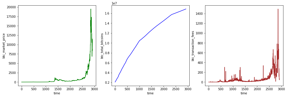
Next, we will plot the three columns of data on three subplots arranged horizontally.
Exercise 6.3
Challenge: Plot line charts for the three columns of
data in the
data
dataset respectively, and arrange them as horizontal
subplots.
Requirement: Set the names of the horizontal and
vertical axes for each chart. The horizontal axis should
be uniformly set to
time, and the vertical axis should be the name of each
column.
Hint: Use
set_xlabel()
to set the name of the horizontal axis.
from matplotlib import pyplot as plt
%matplotlib inline

fig, axes = plt.subplots(1, 3, figsize=(16, 5))

## 代码开始 ### (≈ 9 行代码)


## 代码结束 ###
Solution to Exercise 6.3
from matplotlib import pyplot as plt
%matplotlib inline

fig, axes = plt.subplots(1, 3, figsize=(16, 5))

### Code starts ### (≈ 9 lines of code)
axes[0].plot(data['btc_market_price'], 'green')
axes[0].set_xlabel('time')
axes[0].set_ylabel('btc_market_price')

axes[1].plot(data['btc_total_bitcoins'], 'blue')
axes[1].set_xlabel('time')
axes[1].set_ylabel('btc_total_bitcoins')

axes[2].plot(data['btc_transaction_fees'], 'brown')
axes[2].set_xlabel('time')
axes[2].set_ylabel('btc_transaction_fees')
### Code ends ###
Expected output (color can be ignored)
In this challenge, the features of the dataset are “total number of bitcoins” and “bitcoin transaction fees”, while the target value is “bitcoin market price”. Therefore, the dataset will be split into a training set and a test set below. Among them, the training set accounts for 70%, and the test set accounts for 30%.
Exercise 6.4
Challenge: Split the
data
dataset so that the training set accounts for 70% and
the test set accounts for 30%.
Requirement: The training set features, training set
target, test set features, and test set target are
defined as
X_train,
y_train,
X_test, and
y_test
respectively, and are returned as the return value of
the
split_dataset()
function.
def split_dataset():
    """
    参数:
    无

    返回:
    X_train, y_train, X_test, y_test -- 训练集特征、训练集目标、测试集特征、测试集目标
    """

    ### 代码开始 ### (≈ 6 行代码)

    ### 代码结束 ###

    return X_train, y_train, X_test, y_test
Solution to Exercise 6.4
def split_dataset():
    """
    Parameters:
    None

    Returns:
    X_train, y_train, X_test, y_test -- Training set features, training set target, test set features, test set target
    """

    ### START CODE HERE ### (≈ 6 lines of code)
    train_data = data[:int(len(data)*0.7)]
    test_data = data[int(len(data)*0.7):]

    X_train = train_data[['btc_total_bitcoins', 'btc_transaction_fees']]
    y_train = train_data[['btc_market_price']]

    X_test = test_data[['btc_total_bitcoins', 'btc_transaction_fees']]
    y_test = test_data[['btc_market_price']]
    ### END CODE HERE ###

    return X_train, y_train, X_test, y_test
Run the tests
len(split_dataset()[0]), len(split_dataset()[1]), len(split_dataset()[2]), len(split_dataset()[
    3]), split_dataset()[0].shape, split_dataset()[1].shape, split_dataset()[2].shape, split_dataset()[3].shape
Expected output
(2043,
                      2043,
                      877,
                      877,
                      (2043,
                      2),
                      (2043,
                      1),
                      (877,
                      2),
                      (877,
                      1))
6.4. 3rd Degree Polynomial Regression Prediction Challenge#
After splitting the training data and test data, a polynomial regression prediction model can be constructed. The challenge requires using scikit-learn to complete it.
# 加载必要模块
from sklearn.preprocessing import PolynomialFeatures
from sklearn.linear_model import LinearRegression
from sklearn.metrics import mean_absolute_error

# 加载数据
X_train = split_dataset()[0]
y_train = split_dataset()[1]
X_test = split_dataset()[2]
y_test = split_dataset()[3]
Exercise 6.5
Challenge: Build a 3rd degree polynomial regression prediction model.
Requirement: Use scikit-learn to build a 3rd degree polynomial regression prediction model, calculate the MAE evaluation metric of the prediction results, and return it as the value of the poly3() function.
def poly3():
    """
    参数:
    无

    返回:
    mae -- 预测结果的 MAE 评价指标
    """

    ### 代码开始 ### (≈ 7 行代码)

    ### 代码结束 ###

    return mae
Solution to Exercise 6.5
def poly3():

    """
    Parameters:
    None

    Returns:
    mae -- The MAE evaluation metric of the prediction results
    """

    ### START CODE HERE ### (≈ 7 lines of code)
    poly_features = PolynomialFeatures(degree=3, include_bias=False)
    poly_X_train = poly_features.fit_transform(X_train)
    poly_X_test = poly_features.transform(X_test)

    model = LinearRegression()
    model.fit(poly_X_train, y_train)
    pre_y = model.predict(poly_X_test)

    mae = mean_absolute_error(y_test, pre_y.flatten())
    ### END CODE HERE ###

    return mae
Run the tests
poly3()
Expected output
1955.8027790596564
6.5. Nth Degree Polynomial Regression Prediction Plot#
Next, calculate the corresponding MSE evaluation metric values and plot them for different polynomial degrees.
Exercise 6.6
Challenge: Calculate the MSE evaluation metric for the prediction results of polynomial regression of degrees 1, 2,…, 10.
Requirement: Use scikit-learn to build an Nth-degree
polynomial regression prediction model, calculate the
MSE evaluation metric for the prediction results of
polynomials of degrees 1 - 10, and return it as the
value of the function
poly_plot(N).
from sklearn.pipeline import make_pipeline
from sklearn.metrics import mean_squared_error


def poly_plot(N):
    """
    参数:
    N -- 标量, 多项式次数

    返回:
    mse -- N 次多项式预测结果的 MSE 评价指标列表
    """

    m = 1
    mse = []

    ### 代码开始 ### (≈ 6 行代码)

    ### 代码结束 ###

    return mse
Solution to Exercise 6.6
from sklearn.pipeline import make_pipeline
from sklearn.metrics import mean_squared_error

def poly_plot(N):

    """
    Parameters:
    N -- scalar, degree of the polynomial

    Returns:
    mse -- list of MSE evaluation metrics for the prediction results of the Nth-degree polynomial
    """

    m = 1
    mse = []

    ### START CODE HERE ### (≈ 6 lines of code)
    while m <= N:
        model = make_pipeline(PolynomialFeatures(m, include_bias=False), LinearRegression())
        model.fit(X_train, y_train)
        pre_y = model.predict(X_test)
        mse.append(mean_squared_error(y_test, pre_y.flatten()))
        m = m + 1

    ### END CODE HERE ###

    return mse
Run the tests
poly_plot(10)[:10:3]
Expected output (the results may vary slightly)
[24171680.63629423,
                      23772159.453013,
                      919854753.0234015,
                      3708858661.222856]
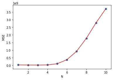
Exercise 6.7
Challenge: Plot the MSE evaluation metric as a line plot
Requirement: Plot the list of MSE returned by
poly_plot(10)
as a combined plot (line plot + scatter plot). Among
them, the line plot is in red.
mse = poly_plot(10)

## 代码开始 ### (≈ 2 行代码)

## 代码结束 ###

plt.title("MSE")
plt.xlabel("N")
plt.ylabel("MSE")
Solution to Exercise 6.7
mse = poly_plot(10)

### Start of code ### (≈ 2 lines of code)
plt.plot([i for i in range(1, 11)], mse, 'r')
plt.scatter([i for i in range(1, 11)], mse)
### End of code ###

### Solution two ###
plt.plot(mse, marker='-o')

plt.title("MSE")
plt.xlabel("N")
plt.ylabel("MSE")
Expected output